

Abstract
Whole-body (WB) dynamic PET has recently demonstrated its potential in translating the quantitative benefits of parametric imaging to the clinic. Post-reconstruction standard Patlak (sPatlak) WB graphical analysis utilizes multi-bed multi-pass PET acquisition to produce quantitative WB images of the tracer influx rate Ki as a complimentary metric to the semi-quantitative standardized uptake value (SUV). The resulting Ki images may suffer from high noise due to the need for short acquisition frames. Meanwhile, a generalized Patlak (gPatlak) WB post-reconstruction method had been suggested to limit Ki bias of sPatlak analysis at regions with non-negligible 18F-FDG uptake reversibility; however, gPatlak analysis is non-linear and thus can further amplify noise. In the present study, we implemented, within the open-source software for tomographic image reconstruction platform, a clinically adoptable 4D WB reconstruction framework enabling efficient estimation of sPatlak and gPatlak images directly from dynamic multi-bed PET raw data with substantial noise reduction. Furthermore, we employed the optimization transfer methodology to accelerate 4D expectation–maximization (EM) convergence by nesting the fast image-based estimation of Patlak parameters within each iteration cycle of the slower projection-based estimation of dynamic PET images. The novel gPatlak 4D method was initialized from an optimized set of sPatlak ML-EM iterations to facilitate EM convergence. Initially, realistic simulations were conducted utilizing published 18F-FDG kinetic parameters coupled with the XCAT phantom. Quantitative analyses illustrated enhanced Ki target-to-background ratio (TBR) and especially contrast-to-noise ratio (CNR) performance for the 4D versus the indirect methods and static SUV. Furthermore, considerable convergence acceleration was observed for the nested algorithms involving 10–20 sub-iterations. Moreover, systematic reduction in Ki % bias and improved TBR were observed for gPatlak versus sPatlak. Finally, validation on clinical WB dynamic data demonstrated the clinical feasibility and superior Ki CNR performance for the proposed 4D framework compared to indirect Patlak and SUV imaging.
Export citation and abstract BibTeX RIS
For more information on this article, see medicalphysicsweb.org
1. Introduction
Molecular imaging involves in vivo visualization, characterization and measurement of biological processes at molecular and cellular levels, often consisting of 2- or 3-dimensional (2D or 3D) imaging as well as quantification over time (Mankoff 2007). Positron emission tomography (PET) is nowadays considered a primary molecular imaging modality capable of quantitatively measuring and localizing radiolabelled biomarkers as they circulate via the blood stream across living tissues (Phelps 2000, Aboagye et al 2001, Gambhir 2002). In particular, static PET employs the established surrogate metric of standardized uptake value (SUV) to evaluate a temporal instantiation of the dynamic in vivo tracer distribution within a single time frame (Wahl and Buchanan 2002).
Dynamic PET, on the other hand, allows for sampling of the time course of the spatial distribution of tracers in the blood (input function) and tissues to enable 4-dimensional (4D) in vivo imaging for a range of molecular biomarkers (Schmidt and Turkheimer 2002, Carson 2005, Bentourkia and Zaidi 2007, Müller-Schauenburg and Reimold 2008). Subsequently, the acquired 4D data may be fitted to a kinetic model to enable quantification of physiological parameters of interest at the individual voxel level, known as parametric PET imaging (Messa et al 1992, Nitzsche et al 1993, Petit-Taboue et al 1996, Gunn et al 1997). Unlike static SUV PET imaging, which only provides a temporal 'snapshot' of the tracer dynamic distribution, parametric PET imaging enables a more objective characterization of the underlying physiology. Thus, the clinical translation of whole-body (WB) dynamic PET imaging may facilitate significant quantitative enhancements in diagnostic, prognostic and theranostic assessments for various oncology, cardiology and neurology diseases.
Nowadays, a wide range of clinical PET imaging protocols involve multi-bed or WB acquisitions to enable assessment of disseminated disease from a single scan session, e.g. assessment of metastatic burden (Wahl and Buchanan 2002). Single-pass or static PET scans can readily support multi-bed field-of-views (FOVs) with sufficient scan time allocated per bed (Kubota et al 1985, Thie 2004, Boellaard et al 2015). On the contrary, extension of current dynamic PET protocols to multi-bed FOVs is more challenging, as it involves multiple WB passes within the same time, resulting in very short scan time frames per bed. Nevertheless, dynamic PET has been steadily garnering clinical interest in oncology for the quantitative assessment of the progress and response to treatment of an increasing range of tumor types (Gupta et al 1998, Prytz et al 2006, Castell and Cook 2008, Kotasidis et al 2014). With the advent of commercial PET scanners with larger axial FOVs, improved electronics, time-of-flight (TOF) and resolution modeling capabilities, studies of higher statistical quality may now be possible in shorter time sessions, paving the way for clinical WB parametric PET imaging (Panin et al 2006, Karp et al 2008, Rahmim et al 2013, Karakatsanis et al 2014b).
Recently, we proposed a clinically adoptable dynamic WB 18F-FDG PET data acquisition framework involving a streamlined 6-pass WB protocol (Karakatsanis et al 2013a, 2013c). In that framework, the dynamic WB PET images were first reconstructed, using a regular 3D maximum-likelihood expectation–maximization (ML-EM) algorithm (Dempster et al 1977, Shepp and Vardi 1982). Then, the standard Patlak (sPatlak) linear graphical analysis method (Patlak et al 1983) was employed on the voxel level to robustly estimate images of the tracer influx rate constant Ki and the blood distribution volume V. As sPatlak considers a linear relationship between the estimated parameters and the measured data, the ordinary least squares (OLS) regression method was applied to robustly fit the images to the model.
Although the sPatlak method is robust and therefore attractive for clinical usage, it does not account for uptake reversibility and therefore it may lead to biased Ki estimates (Hoh et al 2011, Sayre et al 2011). In fact a number of studies have reported mild reversibility for normal tissues (Hawkins et al 1992, Okazumi et al 1992, Fischman and Alpert 1993, Choi et al 1994, Nelson et al 1996, Graham et al 2000, Huang 2000, Zhuang et al 2001, Iozzo et al 2003, Lin et al 2005, Prytz et al 2006) as well as some oncologic malignancy types, such as hepatocellular carcinoma (HCC) tumors (Messa et al 1992, Torizuka et al 1995). As such, we recently proposed the non-linear generalized Patlak (gPatlak) WB imaging method which utilizes the additional net efflux rate constant kloss to account for mild uptake reversibility and thus reduce the observed sPatlak Ki bias in multiple bed positions (Karakatsanis et al 2015a).
Both above-mentioned techniques are conducted at the image level as a separate post-reconstruction step and, therefore, are characterized as indirect parametric imaging methods. Since each dynamic frame is reconstructed separately from the rest, the counts contributing to each dynamic image are limited to the respective time frame thus enhancing noise levels in the estimates. Alternatively, parametric PET images can be reconstructed directly from the complete set of dynamic raw PET measurements as initially introduced by Matthews et al (1997). Interested readers may refer to informative literature reviews on the topic (Tsoumpas et al 2008a, 2008b, Rahmim et al 2009, Wang and Qi 2013, Kotasidis et al 2014, Reader and Verhaeghe 2014). In particular, the sPatlak model has been previously incorporated within the ML-EM framework to enable direct estimation of Ki and V macro-parameters from dynamic single-bed PET raw data (Tsoumpas et al 2008a, Wang and Qi 2009, Tang et al 2010, Verhaeghe and Reader 2010). Unlike post-reconstruction Patlak analysis, 4D Patlak algorithms allow for direct ML-EM estimation from the complete 4D dataset, performing comprehensive counts utilization. In addition, the statistical noise in the raw data follows the well-known Poisson distribution, which can be accurately modeled within 4D reconstruction algorithms, while the indirect methods commonly oversimplify the complex noise distribution in the reconstructed PET images (Barrett et al 1994, Qi 2003, Rahmim and Tang 2013, Reader and Verhaeghe 2014). Therefore, 4D Patlak reconstruction is expected to yield reduced noise levels than indirect methods, with the difference becoming more apparent for low count statistics.
Due to a higher model complexity in 4D reconstruction, a larger number of iterations are needed for the convergence of the image estimates (Wu 1983, Kamasak et al 2005, Rahmim et al 2009). Moreover, the convergence rate may be further decelerated due to inherent correlations between the Patlak temporal basis functions (Wang et al 2008, Tsoumpas et al 2008b, Rahmim et al 2009, Tang et al 2010, Wang and Qi 2010, Karakatsanis et al 2013b). As a result, the slower tomographic update is interleaved with the faster Patlak update at each iterative step. Alternatively, the principle of optimization transfer (Carson and Lange 1985, Lange et al 2000) can be employed to define surrogate objective functions, which in turn allow for nesting of multiple sub-iterations of the fast image-based ML-EM update process within each global iteration of the slower projection-based ML-EM update (Wang and Qi 2010, 2012, 2013, Karakatsanis and Rahmim 2014a). The same principle has been also employed for the integration of resolution (Angelis et al 2013) and motion (Karakatsanis et al 2014d) models within PET image reconstruction. As the image-based Patlak ML-EM sub-iterations are considerably faster than the external tomographic ML-EM global iterations, multiple Patlak updates can be accommodated within each global iteration, thus facilitating convergence at a negligible computational cost per global iteration.
In the meantime, Zhu et al (2012, 2014) developed a non-nested 4D sPatlak algorithm for direct reconstruction from list-mode data across multiple beds. Their approach was based on a simplified 2-pass WB dynamic protocol (dual-time Patlak), which may be the minimum necessary number of passes to estimate the two sPatlak parameters (slope and intercept) but not for non-linear gPatlak regression involving 3 parameters. Furthermore, the choice of two WB passes does not offer any redundancy if the initial scan window is not found to be optimal for the evaluated tracer kinetics (Karakatsanis et al 2014c) or if the patient chooses to suddenly stop the exam before the two passes are completed.
Here we propose a multi-bed extension of the previous nested 4D sPatlak algorithms to directly and efficiently reconstruct sPatlak WB images from dynamic WB PET raw data at an accelerated convergence rate. In addition, we present a novel non-linear 4D nested gPatlak reconstruction algorithm for quantitative WB Ki imaging either in single- or multi-bed FOVs, including regions where linear sPatlak yields biased Ki estimates, due to non-negligible uptake reversibility. Both methods are based on our previously optimized 6-pass WB scan protocol corresponding to 0–45 min post injection (p.i.) scan window. By acquiring six WB passes, the necessary temporal data redundancy is attained to facilitate (a) kinetic-driven optimization of the acquisition time window, and (b) robust estimation of Patlak parametric images, especially for gPatlak non-linear parameters. Finally, we introduce a practical sPatlak-based initialization scheme for the gPatlak 4D algorithm to potentially overcome convergence problems to local optima, due to high noise in the data (Wu 1983). All proposed and reference algorithms have been implemented and validated on the open-source Software for tomographic image reconstruction (STIR) platform (Thielemans et al 2012) by building upon existing non-nested sPatlak reconstruction libraries (Tsoumpas et al 2008a) and including both simulated and clinical studies. As we target clinical adoptability, we laid emphasis on efficiency, robustness and application scope for the proposed methods.
2. Materials and methods
2.1. Whole-body dynamic PET acquisition protocol
The proposed WB dynamic PET data acquisition protocol consists of an initial dynamic PET scan at the cardiac bed position, immediately following tracer administration (first phase), namely 0–6 min p.i., to measure the rapidly changing early section of the tracer concentration in the blood plasma (input function). Then, a dynamic series of 6 WB passes follows (second phase), for 8–45 min p.i. (figure 1), to sample the later part of the tissue time activity curves (TACs) at every voxel across the WB FOV. The protocol has been streamlined for straightforward clinical adoption: each dynamic WB frame is scanned along the same axial direction (cranio-caudal or vice versa) and consists of equal number of beds of equal duration resulting in uniform temporal sampling rates for all bed positions (Karakatsanis et al 2013a).

Figure 1. Flow chart illustrating the sequence of all dynamic bed frames, as acquired with the step-and-shoot mode during the 2nd phase of the suggested WB dynamic PET protocol. In the example, 6 unidirectional (cranio-caudal) WB passes are acquired, each comprised of 7 beds of equal scan duration. Later the parametric Ki image at each column, i.e. bed position, is directly estimated via 4D sPatlak and gPatlak algorithms from the image-derived input function and the respective dynamic projection PET data.
Download figure:
Standard image High-resolution imageInitially, the PET 4D raw data from both protocol phases are independently reconstructed and the input function is extracted from regions-of-interest (ROIs) placed over the heart left-ventricle (LV) in the resulting PET dynamic images. The ROIs are drawn such that partial volume effects are minimized (Karakatsanis et al 2013a). Subsequently, the image-derived input function is utilized to produce WB parametric Ki images with (a) our previously validated indirect Patlak analysis and (b) the newly proposed direct 4D Patlak reconstruction methods.
2.2. Patlak graphical analysis methods
2.2.1. Linear standard Patlak (sPatlak) graphical analysis.
In multi-bed dynamic PET acquisitions, the linear sPatlak graphical analysis method (Patlak et al 1983) utilizes the dynamic PET data from each bed position and the input function to estimate the kinetic macro-parameters of tracer influx rate constant  , in units of ml of blood per minute per gram of tissue (ml (min × g)−1), and total distribution volume
  , in units of ml of blood per gram of tissue (ml g−1), at each voxel (Karakatsanis et al 2013a):
where  denotes the convolution operation over the time variable t' and
  is the measured tissue TAC at the mid-frame time points
  of the
  dynamic PET frames, corresponding to a particular bed and voxel. Moreover,
  is the input function at the
  time points and
  is the p.i. time after which relative kinetic equilibrium between the blood and the tissue tracer concentration is attained. The sPatlak analysis assumes an irreversible 2-tissue-compartment tracer kinetic model, as illustrated in figure 2(a).
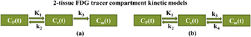
Figure 2. Standard 2-tissue compartment 18F-FDG kinetic models (a) without and (b) with uptake reversibility constant rate k4. The CP, Ce and Cm compartments denote the activity concentration in blood plasma and in tissue exchangeable and metabolized states, respectively (Gunn et al 2001).
Download figure:
Standard image High-resolution imagePatlak and Blasberg (1985) showed that the macro-parameter  can be related to the kinetic micro-parameters
  (ml (min × g)−1),
  (min−1),
  (min−1) and
  (min−1) as follows:

2.2.2. Non-linear generalized Patlak (gPatlak) graphical analysis.
Standard linear Patlak analysis directly estimates Ki and V macro-parameters by assuming a 2-tissue-compartment kinetic model with an irreversible compartment, a commonly invoked model for organs and tumors exhibiting 18F-FDG uptake in PET human studies (Gunn et al 2001). However a considerable number of studies suggest uptake reversibility for a range of tracers, as presented previously (Holden et al 1997, Lodge et al 1999, Karakatsanis et al 2015a). Since the sPatlak model assumes irreversible uptake, it may underestimate Ki to compensate for lack of reversibility modeling (Messa et al 1992, Hoh et al 2011, Sayre et al 2011).
Therefore, later Patlak and Blasberg (1985) introduced a generalized graphical analysis method to account for mildly reversible uptake kinetics. A  kinetic parameter was introduced to describe the net rate constant for absorbed or metabolized tracer loss to the blood plasma. By assuming a reversible 2-tissue compartment model with
  , it follows (Karakatsanis et al 2015a):
The net efflux rate constant  (min−1) is related to the kinetic micro-parameters as follows:

Despite the presence of a non-linear term in equation (3), gPatlak analysis is characterized by a significantly lower degree of complexity and, thus higher robustness, than the standard 2-tissue compartmental kinetic modeling methods. Nevertheless, gPatlak is less robust to noise, but enhances  quantification in voxels with uptake reversibility, compared to sPatlak analysis (Karakatsanis et al 2015a).
2.3. Direct 4D WB Patlak imaging
Previously, we proposed a set of indirect WB PET parametric imaging tools utilizing either sPatlak or gPatlak graphical analysis (Karakatsanis et al 2013a, 2015a), here denoted, in general, as (s/g)Patlak methods. The standard OLS and the basis function method (BFM) (Gunn et al 1997) were then applied on the reconstructed dynamic PET images to estimate the sPatlak and gPatlak parameters respectively. However, the main scope of the current study is the design and validation of clinically adoptable direct 4D (s/g)Patlak ML-EM WB reconstruction methods for more efficient utilization of the 4D data, at each bed position, when estimating kinetic macro-parameters.
2.3.1. Nested direct 4D WB sPatlak reconstruction.
Let us first define the following:
![$\boldsymbol{y}^{{n}}=\left[\,y_{i}^{n}\right]_{i=1}^{I}$](data:image/png;base64,iVBORw0KGgoAAAANSUhEUgAAAAEAAAABCAQAAAC1HAwCAAAAC0lEQVR42mNkYAAAAAYAAjCB0C8AAAAASUVORK5CYII=) : nth dynamic frame of a PET sinogram or projection data vector comprised of a total of detector pair or line-of-response (LOR) bins,
: nth dynamic frame of a PET sinogram or projection data vector comprised of a total of detector pair or line-of-response (LOR) bins,- : column vector of a set of dynamic frames of measured PET sinograms,
- : nth dynamic frame of a PET image vector comprised of a total of voxels,
- : column vector of a set of dynamic frames of reconstructed PET images,
- : parametric image vector of the Patlak slope or tracer influx rate constant ,
- : parametric image vector of the Patlak intercept or blood distribution volume ,
- : ensemble standard Patlak parametric image vector
- : measured blood plasma activity concentration at mid-frame time ,
- : integral of along time variable
- : spatial system response matrix with denoting the probability an annihilation event having occurred at jth image voxel to be recorded at ith detector pair or line or response (LOR) of the sinogram, thus ,
- : standard Patlak model matrix and
- : spatio-temporal system response matrix derived by taking the Kronecker product of P and Bs model response matrices.
![$\boldsymbol{y}^{{n}}=\left[\,y_{i}^{n}\right]_{i=1}^{I}$](https://content.cld.iop.org/journals/0031-9155/61/15/5456/revision1/pmbaa2c08ieqn019.gif)

![$\boldsymbol{Y}={{\left[\,\boldsymbol{y}^{{1}}\ldots \boldsymbol{y}^{{N}}\right]}^{T}}$](https://content.cld.iop.org/journals/0031-9155/61/15/5456/revision1/pmbaa2c08ieqn021.gif)

![$\boldsymbol{x}^{{n}}=\left[x_{j}^{n}\right]_{j=1}^{J}$](https://content.cld.iop.org/journals/0031-9155/61/15/5456/revision1/pmbaa2c08ieqn023.gif)

![$\boldsymbol{X}={{\left[\boldsymbol{x}^{{1}}\ldots \boldsymbol{x}^{{N}}\right]}^{T}}$](https://content.cld.iop.org/journals/0031-9155/61/15/5456/revision1/pmbaa2c08ieqn025.gif)

![$\boldsymbol{K}=\left[K_{\text{i}}^{j}\right]_{j=1}^{J}$](https://content.cld.iop.org/journals/0031-9155/61/15/5456/revision1/pmbaa2c08ieqn027.gif)

![$\boldsymbol{V}=\left[{{V}^{j}}\right]_{j=1}^{J}$](https://content.cld.iop.org/journals/0031-9155/61/15/5456/revision1/pmbaa2c08ieqn029.gif)

![$\boldsymbol{M}_{{s}}={{\left[\boldsymbol{K}\text{;}\boldsymbol{V}\right]}^{T}}$](https://content.cld.iop.org/journals/0031-9155/61/15/5456/revision1/pmbaa2c08ieqn031.gif)


![$\boldsymbol{P}=\left[\,{{p}_{ij}}\right]_{i=1,j=1}^{I,J}$](https://content.cld.iop.org/journals/0031-9155/61/15/5456/revision1/pmbaa2c08ieqn037.gif)


![$\boldsymbol{B}_{{s}}=\left[{{b}_{s,nk}}\right]_{n=1,k=1}^{N,2}=\left[\begin{array}{c} {{S}_{\text{P}}}(1) & {{C}_{\text{P}}}(1) \\ \vdots & \vdots \\ {{S}_{\text{P}}}(N) & {{C}_{\text{P}}}(N) \end{array}\right]$](https://content.cld.iop.org/journals/0031-9155/61/15/5456/revision1/pmbaa2c08ieqn040.gif)
![$\overline{\boldsymbol{P}}=\left[\begin{array}{c} {{S}_{\text{P}}}(1)\boldsymbol{P} & {{C}_{\text{P}}}(1)\boldsymbol{P} \\ \vdots & \vdots \\ {{S}_{\text{P}}}(N)\boldsymbol{P} & {{C}_{\text{P}}}(N)\boldsymbol{P} \end{array}\right]=\boldsymbol{P}\oplus \boldsymbol{B}_{{s}}$](https://content.cld.iop.org/journals/0031-9155/61/15/5456/revision1/pmbaa2c08ieqn041.gif)

According to standard Patlak graphical analysis, the expectations of dynamic sinograms ![$\widehat{\boldsymbol{Y}}={{\left[{{\widehat{\boldsymbol{y}}}^{1}}\ldots {{\widehat{\boldsymbol{y}}}^{N}}\right]}^{T}}$](https://content.cld.iop.org/journals/0031-9155/61/15/5456/revision1/pmbaa2c08ieqn043.gif) and respective PET images
and respective PET images ![$\widehat{\boldsymbol{X}}={{\left[{{\widehat{\boldsymbol{x}}}^{1}}\ldots {{\widehat{\boldsymbol{x}}}^{N}}\right]}^{T}}$](https://content.cld.iop.org/journals/0031-9155/61/15/5456/revision1/pmbaa2c08ieqn044.gif) can be directly related to the expected ensemble parametric image
can be directly related to the expected ensemble parametric image ![${{\widehat{\boldsymbol{M}}}_{s}}={{\left[\widehat{\boldsymbol{K}};\widehat{\boldsymbol{V}}\right]}^{T}}$](https://content.cld.iop.org/journals/0031-9155/61/15/5456/revision1/pmbaa2c08ieqn045.gif) of tracer influx rate constant
of tracer influx rate constant  and blood distribution volume
  according to the following linear kinetic model equations:

or, equivalently:

Then the two 4D maximum likelihood expectation–maximization (ML-EM) update equation follows:
or, equivalently:

By letting ![$\boldsymbol{m}_{s}^{j}=\left[m_{s,k}^{j}\right]_{k=1}^{2}={{\left[K_{i}^{j}{{V}^{j}}\right]}^{T}}$](https://content.cld.iop.org/journals/0031-9155/61/15/5456/revision1/pmbaa2c08ieqn048.gif) as the standard Patlak parameter vector at voxel
as the standard Patlak parameter vector at voxel  , we have:
The nested 4D sPatlak image reconstruction algorithm breaks down the previous integrated EM process into two steps: (i) a single tomographic projection-based EM update of the dynamic image estimates, based on the measured 4D data, followed by (ii) multiple nested image-based EM updates of the kinetic parameter estimates, based on the dynamic image estimates from step 1. The nested ML-EM implementation utilizes the 'optimization transfer' principle (Lange et al 2000), which 'transfers' the optimization target from a single and more complex global objective function to simpler surrogate functions, that vary at each global ML-EM iteration step, as illustrated in figure 3 (Carson and Lange 1985, Wang and Qi 2010, 2012, 2013, Karakatsanis and Rahmim 2014a).
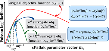
Figure 3. (Left) Diagram of ML-EM global objective function  (red curve) and surrogate functions
  (blue) and
  (green) for global iterations
  and
and  , respectively. They all are Poisson log-likelihood functions depending on the sPatlak parameter vector
  . The basic principles of optimization transfer are illustrated as follows: (a) each value of the
  th surrogate function is either lower or equal to the value of the global objective function at the same
  . In addition, (b) the maximum value of
  th surrogate function is equal to the value of the global function at
  . The set of parameters maximizing the
  th surrogate objective function is considered the optimal for
  th iteration, as described in (c). Finally,
  yields higher values for the global objective function, as the iterations progress (d).
Download figure:
Standard image High-resolution imageIn the nested sPatlak 4D ML-EM framework, both the global objective function  and the surrogate objective function
  , for each iteration
  , are defined as Poisson log-likelihood functions of the measured dynamic data Y and the dynamic image estimate xw at iteration
  , respectively, given the sPatlak parameter vector
  . In fact, the nested section of the sPatlak 4D ML-EM algorithm for global iteration
  utilizes the latest dynamic image estimate xw from step 1 to return, after several sub-iterations, the ms parameter vector that maximizes the
  th iteration surrogate log-likelihood function
  (figure 3(c)). Subsequently, the returned value
  initializes the tomographic ML-EM update (step 1) of the next, i.e.
  th iteration.
We note that our scheme employs an ML-EM optimization algorithm for both the external tomographic and the nested image-based iterative update processes, while the respective Poisson log-likelihood functions satisfy the criteria described in figures 3(a) and (b). In addition, the external and nested Poisson log-likelihood maximization problems described above are equivalent to minimizing the Kullback–Leibler (KL) distance metrics (Barrett and Myers 2004) between the measured dynamic data Y and dynamic images xw, for the tomographic estimation problem, and between the estimated dynamic images xw and the new sPatlak parameter estimates  for the image-based parametric estimation problem. Under these conditions, the 4D ML-EM nested estimation of the sPatlak parameters is legitimately performed, as the Poisson distribution in the measured counts is fully accounted, and the EM convergence of the nested 4D ML-EM algorithm is ensured, as illustrated in figure 3(d).
Below, we present the theoretical framework of the nested sPatlak 4D ML-EM algorithm (Wang and Qi 2010). In this work, we extended its application to raw PET data from multiple beds. Initially, for every global ML-EM iterative cycle, an updated dynamic image set  is estimated for each bed utilizing the large tomographic system matrix P and the respective bed dynamic data Y (step 1):

or, equivalently:
Subsequently, the algorithm performs a series of nested ML-EM updates of the kinetic parameter images K and V, corresponding to each bed, by employing the considerably smaller in size sPatlak model matrix  and the respective PET image estimates
  from step 1 as a reference (step 2):
or, equivalently:
Then, the nested sPatlak 4D ML-EM steps above are repeated for the data of the remaining beds to produce the respective sPatlak images. Finally, all images of the same parameter type are combined, after accounting for any axial overlapping slices between beds, to create multi-bed or WB sPatlak images.
The first step of each global EM iteration cycle involves forward- and back-projection 3D tomographic operations, which are often computationally expensive due to the large size of P. On the contrary, the nested EM loop of the second step employs the much smaller model matrix Bs, thus allowing for much faster forward- and back-projection operations to transform between parametric and dynamic image space. Thus, by nesting multiple faster update steps of the kinetic parameter estimates (equations (9a) and (9b)) within every tomographic update step of the dynamic images (equation (8a) or (8b)), the global convergence rate of the 4D reconstruction algorithm is effectively accelerated, in terms of total computation time (Wang et al 2010, Wang and Qi 2013, Karakatsanis and Rahmim 2014a).
2.3.2. Nested direct 4D WB gPatlak reconstruction.
For the non-linear gPatlak model let us denote:
- K, kloss and V: column vectors denoting respective , and parametric images,
- : the overall gPatlak parametric image matrix,
- : vector of the three gPatlak parameters at voxel ,
- : variable denoting each of the convolution time points (different from , variable for the mid-frame time points)
- : gPatlak impulse response element at time point for voxel ,
- : impulse response column vector at voxel and
- : TAC at voxel .


![$\boldsymbol{M}_{{g}}={{\left[\boldsymbol{K};\boldsymbol{k}_{{\text{loss}}};\boldsymbol{V}\right]}^{T}}$](https://content.cld.iop.org/journals/0031-9155/61/15/5456/revision1/pmbaa2c08ieqn080.gif)


![$\boldsymbol{h}^{{j}}=\left[h_{d}^{j}\right]_{d=1}^{D}$](https://content.cld.iop.org/journals/0031-9155/61/15/5456/revision1/pmbaa2c08ieqn090.gif)

![$\boldsymbol{x}_{{j}}=\left[x_{j}^{n}\right]_{n=1}^{N}$](https://content.cld.iop.org/journals/0031-9155/61/15/5456/revision1/pmbaa2c08ieqn092.gif)

According to gPatlak model assumptions in (3) the TAC at every voxel  can be modeled as follows:

By approximating the above time convolution operation with a summation over  finely sampled time convolution points
  , we can also model every voxel TAC
  as a vector-matrix product:

where ![$\boldsymbol{r}^{{j}}={{\left[\boldsymbol{h}^{{j}};{{V}^{j}}\right]}^{T}}$](https://content.cld.iop.org/journals/0031-9155/61/15/5456/revision1/pmbaa2c08ieqn098.gif) is the Patlak response vector at voxel
is the Patlak response vector at voxel  , constructed by appending the
  unknown parameter at the end of the impulse response vector
  , and
, and  is the
  matrix derived from the Toeplitz matrix (Heinig and Ross 1984) of
  for
for  temporal convolution points:
For the proposed nested gPatlak 4D ML-EM WB reconstruction algorithm, each global iteration step is now decomposed into three distinct respective steps, unlike the two steps previously described for nested sPatlak 4D algorithm.
The first step, which is identical with step 1 of the nested sPatlak 4D method, involves a single update of the estimated TAC ![$\boldsymbol{x}_{{j}}=\left[x_{j}^{n}\right]_{n=1}^{N}$](https://content.cld.iop.org/journals/0031-9155/61/15/5456/revision1/pmbaa2c08ieqn106.gif) at voxel
at voxel  , through a tomographic EM estimation process, and is often the most computationally expensive, as it is applied consecutively to all
  dynamic frames and employs the large tomographic matrix P. Thus, for
  and
and  , we have for step 1:
Subsequently, the previously estimated TAC  of voxel j from step 1 and the measured data in
  are employed to estimate the Patlak response vector
  of size
  , through the following nested iterative ML-EM process (step 2):
Thus, after all nested sub-iterations in step 2 of current global iteration have been completed,  is estimated, which includes the impulse response vector hj and gPatlak parameter
  . Subsequently, in step 3 of current global iteration, the gPatlak parameters
  and
and  are analytically derived, as it will be described later. By repeating the previous 3 steps for a number of ML-EM iterations in all voxels of a particular bed position, the gPatlak images are reconstructed for that bed. Finally, this process is repeated for the dynamic data of the rest of the beds, to ultimately produce WB gPatlak images.
Similarly with sPatlak, the presented nested gPatlak 4D algorithm targets at Poisson log-likelihood types of global and surrogate functions and employs the ML-EM algorithm for the external and the nested optimization problems. The main difference lies in the type of nested estimates targeted by the gPatlak algorithm. Due to the non-linear relationship between the gPatlak parameters and dynamic image space, the latter could not be estimated directly from the nested ML-EM approach employed in the previous section for nested sPatlak 4D case. Instead, the Patlak response vector rj at each voxel j is now estimated through the same nested ML-EM update process, as it is linearly related with the dynamic image estimates, according to equation (10b). Therefore, the same conditions apply to gPatlak case, as those illustrated in figure 3, if sPatlak parameter vector ms is replaced by the Patlak impulse response vector r. In fact, if kloss is set to zero, the gPatlak 4D formulation in equation (10b) reduces to the sPatlak framework and the direct linear relationship between parametric and dynamic image space is restored.
The updated Patlak response vector rj maximizes now a surrogate Poisson log-likelihood given the current TAC estimate xj from step 1, as illustrated below:
The first parameter to be updated at every nested ML-EM iteration of equation(13) is  , as the last element of the updated vector rj. Then, inspired by a similar analytical derivation for a reversible 1-tissue compartment kinetic model (Yan et al 2012, Wang and Qi 2013), the analytical solutions for K and kloss gPatlak parameters at every voxel j can be calculated as follows (Karakatsanis and Rahmim 2014a):
where  is the inverse of the function below:
In order to enhance computational efficiency, a look-up table for  can be pre-calculated and loaded to computer memory at the start of the reconstruction algorithm for a range of possible
  initial values. Then, during reconstruction, this look-up table can be utilized to invert
  function and efficiently determine the updated estimate
  with equation (15).
Finally, the tracer influx rate constant parameter  can be also analytically calculated from the current estimates
  and
and  as follows:
Although the  look-up table is pre-loaded, the estimation of gPatlak parameters
  and
and  from the current rj estimate may be computationally inefficient, if repeated for each nested sub-iteration. Besides, only the EM update of rj is strictly required to maximize the surrogate EM log-likelihood as in equation (14). Therefore, here we propose updating only the rj vector at every nested sub-iteration, except for the last one wherein the gPatlak parameters
  and
and  are estimated as well.
Furthermore, we recommend not using the newly estimated  and
and  parameters to update
  estimates of the new global iteration cycle. Aside from the observation that such an update would be redundant and only add computational cost, as
  is already updated before, it can also be 'risk-prone' for the proper global EM convergence of the algorithm. The risk lies in the estimation of
  and
and  parameters, which is not exclusively driven by the nested ML-EM process (steps 1 and 2), as was the case with sPatlak 4D method. Now, an analytical derivation is additionally employed in the end (step 3), which forces the new estimates
  and
and  to be related with
 ![$\boldsymbol{h}^{{j}}=\left[h_{d}^{j}\right]$](https://content.cld.iop.org/journals/0031-9155/61/15/5456/revision1/pmbaa2c08ieqn141.gif) according to the following equation:
according to the following equation:  ,
,  , provided
  inversion in equation (15) is accurate. Therefore, depending on the sampling density of the
  discrete look-up table and its range (equation (16)), which can both be freely determined by the user, the linear interpolation accuracy of
  inversion in equation (16) may be degraded, therefore affecting the bias in the parametric
  and
and  estimates. As a result, the optimization transfer requirements may not be strictly fulfilled, if the inversion of the
  look-up table is interfering with ML-EM estimation at every global iteration step. Although we have observed a negligible error associated with the analytic calculations even when moderate sampling rates are selected (1000 samples uniformly drawn from a (10−5,1) kloss range), the overall convergence of the ML-EM algorithm may nevertheless be affected after several global ML-EM iterations. Therefore, to ensure the proper EM convergence properties of the gPatlak 4D algorithm and save computational time, the rj vector of the next global tomographic iteration in equation (12) should be updated directly from the rj estimate of the last nested sub-iteration, denoted as
  in equation(13).
2.3.3. Initialization schemes of the 4D Patlak reconstruction methods.
Normally, conventional 3D ML-EM iterative reconstruction algorithms are associated with objective functions that do not require any special initialization scheme. In this study, all 3D ML-EM methods have been initialized with unity values. The sPatlak 4D algorithms are also characterized by a sufficiently stable EM convergence when initialized with unity Ki and V images, due to their linearity and robustness, and thus no special initialization was applied to this class of methods.
Nevertheless, non-linear 4D reconstruction methods involve more complex objective functions, and a more advanced initialization scheme may be helpful. In particular, gPatlak 4D algorithms involve non-linear parameters, and thus, their EM convergence is sensitive to initialization. Therefore, for gPatlak 4D nested algorithm we evaluated (i) a conventional scheme involving initialization of Ki and V estimates with unity values, and (ii) a novel sPatlak-based scheme, where Ki and V parameters were initialized with respective sPatlak 4D estimates. In both cases, kloss initial value was set to zero, which is equivalent to the sPatlak method. Although initialization with zero values is not recommended in ML-EM algorithms to avoid trapping of estimates to zeroes in subsequent iterations due to the multiplicative update mechanism, kloss belongs to an exponential term in the gPatlak model and thus zero is effectively translated as the unity value. The number of sPatlak ML-EM iterations employed to produce the parameter values for gPatlak initialization were determined based on noise-bias trade-off performance in simulated data.
2.4. Design of simulation study and image reconstruction strategy
For the purposes of the simulation study, we initially modeled a set of realistic TACs for various characteristic regions of the human body by employing FDG kinetic parameters from literature (table 1), assuming Feng input function model (Feng et al 1993) and a reversible 2-tissue-compartment model.
Table 1. Published 18F-FDG kinetic parameter values for simulations (Okazumi et al 1992, 2009, Torizuka et al 1995, 2000, Dimitrakopoulou-Strauss et al 2006).
| Regions | k1 (ml (min × g)−1) | k2 (l min−1) | k3 (l min−1) | k4 (l min−1) | Vb (ml ml−1) |
|---|---|---|---|---|---|
| Normal liver | 0.864 | 0.981 | 0.005 | 0.016 | — |
| Liver tumor | 0.243 | 0.78 | 0.1 | 0.002 | — |
| Normal lung | 0.108 | 0.735 | 0.016 | 0.013 | 0.017 |
| Lung tumor | 0.301 | 0.864 | 0.097 | 0.001 | 0.168 |
| HCC tumor | 0.283 | 0.371 | 0.057 | 0.012 | |
| Myocardium | 0.6 | 1.2 | 0.1 | 0.001 | — |
Note: Vb denotes the blood volume fraction in tissue. Tumor kinetic parameter values may correspond to primary or metastatic malignancies in the respective region.
Then, a dynamic series of noise-free emission images were generated by assigning the modeled TACs to the respective regions of a voxelized XCAT human torso digital phantom at the time frames of the proposed protocol (figure 1). A total of six tumor regions were also added: three in the normal liver (A1, A2 and A3) and three in the right lung (B1, B2 and B3) background regions, with the members of each group having diameters in descending order of 15, 10, and 8 mm, respectively. Finally, tumor groups A and B were assigned the kinetics of liver and HCC metastatic tumors, respectively (table 1).
Later, analytic simulations were conducted by forward projecting the emission images with STIR (Thielemans et al 2012) using the Biograph mCT system geometry (Jakoby et al 2011). Then, the generated sinograms were attenuated, according to the XCAT attenuation factors, and scaled based on a factor accounting for the sensitivity of the mCT scanner and the time frame duration. Quantitative Poisson noise was then added. Finally, the generated noise-free and noisy dynamic PET projection data were all reconstructed in either 3D or 4D mode, using current and newly developed STIR ML-EM libraries to produce dynamic PET and Patlak parametric images, respectively. A diagram illustrating the design of the simulated study, along with examples of reconstructed Patlak images, is presented in figure 4.
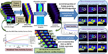
Figure 4. Diagram illustrating the steps for generating realistic simulation data of quantitative levels of noise and the subsequent reconstruction analysis to compare direct 4D versus indirect (s/g)Patlak imaging methods.
Download figure:
Standard image High-resolution imageFor the evaluation of the 4D simulated data, ground truth kinetic parameters were known. Thus, the quantitative analysis was first conducted in terms of percentage (%) normalized bias (NBias × 100) and normalized standard deviation or noise (NSD × 100), where NBias and NSD were calculated over  simulated realizations, according to Karakatsanis et al (2013a), paragraph 4.2. Both metrics were extracted from four characteristic tumor regions (A1, A2, B1 and B2), as a function of the number of ML-EM iterations and plotted together to form noise-bias trade-off curves for each ROI and evaluated method. In addition, we assessed the mean target to background (TBR) and contrast to noise ratio (CNR) metrics for the same tumor regions after averaging over the 20 realizations, according to equations (18) and (19) below.


where  and
and  are the mean values over the target (tumor) and background (normal organ) ROIs, respectively, for
  realization, and
  is the spatial standard deviation of the background ROI, as defined in Karakatsanis et al (2013a), paragraph 4.2.
For the clinical validation, the Siemens Biograph mCT PET/CT scanner (Jakoby et al 2011) was used together with the validated scan protocol described in section 2.1. A set of 5 clinical WB dynamic datasets have been reconstructed with the presented methods. As STIR currently supports only non-TOF projectors, the mCT TOF PET raw data were first converted to a non-TOF format. Two suspected tumor regions of high focal uptake were identified to assess the clinical feasibility and quantitative performance of direct 4D WB Patlak imaging methods against conventional SUV and indirect Patlak analysis in clinical oncology. In all cases, the TBR and CNR scores were evaluated, as a function of the ML-EM global iterations, according to equations (18) and (19) for  .
.
In this study we chose to evaluate the effect on convergence of non-nested versus nested algorithms in the context of a pure ML-EM framework, i.e. by utilizing data from all projection angles at every update cycle of the reconstruction algorithm. Thus, we were able to maintain a common framework to enable direct comparison with previous related ML-EM evaluation work on WB Patlak Ki clinical imaging studies (Karakatsanis et al 2013a, 2013c, 2015a). In addition, we isolated the effects on convergence from other factors, such as that of ordered subsets EM (OS-EM) implementations, which are also expected to accelerate convergence by subsetizing projections at each update cycle. Nevertheless, STIR platform also supports OS-EM algorithm and our preliminary results indicate the same degree of convergence acceleration between nested ML-EM and nested OS-EM when 21 subsets are employed for the latter, which is the standard selection for most clinical studies with the mCT scanner.
3. Results
3.1. Performance evaluation from 4D simulations
3.1.1. Noise-free direct 4D versus SUV imaging.
The noise-free dynamic PET SUV cardiac images in figure 5(a) (1st row) illustrate the variability introduced to each simulated lesion uptake and contrast during the first 45 min p.i. due to the modeled kinetics (table 1). The simulated dynamic PET images were produced from 3D ML-EM reconstruction (3 cycles of 21 iterations each) of dynamic cardiac data which were sampled according to our validated WB dynamic PET protocol (figure 1). Moreover, the reconstructed noise-free indirect and direct (s/g)Patlak Ki images in the 2nd row of figure 5(a) converged to higher lesion TBR contrast scores than any of the dynamic noise-free PET images for both ROI groups A and B. Therefore, in the absence of noise, Patlak may theoretically offer information beyond SUV and thus the complementary application of the two may enhance lesion detectability performance.
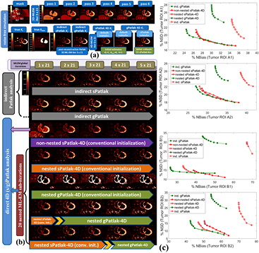
Figure 5. (a) Overview of noise-free Ki and kloss images and (b) noisy Ki images from simulated 4D PET data employing indirect and direct (s/g)Patlak methods. The orange and green bars denote sPatlak and gPatlak ML-EM global iterations respectively for the images directly above. In the last 2 rows, the yellow arrow position between the two bars designates at which iteration were the gPatlak estimates, on the right, initialized from the sPatlak estimates, on the left. (c) Quantitative Ki noise-bias trade-off analysis on four ROIs across 20 noise realizations. The red and green colors correspond to sPatlak and gPatlak methods, while the continuous and dotted delineations indicate direct and indirect methods, respectively. The triangle markers on red curves denote non-nested sPatlak method. Evaluations were conducted every 21 global ML-EM iterations, each consisting of 20 nested sub-iterations. Thus, gPatlak-4D was initialized after 3 × 21 = 63 sPatlak ML-EM iterations.
Download figure:
Standard image High-resolution image3.1.2. Direct 4D versus indirect (s/g)Patlak WB imaging.
In noise-free conditions, indirect and direct methods are expected to match in performance, after convergence is attained. Indeed, no visually distinct difference was observed in the noise-free Ki images between the two method classes (figure 5(a)). In the presence of noise, however, the benefit in noise and resolution of properly initialized direct 4D versus indirect Patlak analysis is illustrated when visually comparing the noisy Ki simulated images (figures 4 and 5(b)), especially for the tumor lesions of B group in the right lung. Moreover, the noise-bias trade-off curves (figure 5(c)) clearly demonstrated, for all evaluated ROIs, the superiority of 4D sPatlak and properly initialized 4D gPatlak algorithms, relative to the respective indirect methods. In particular, we observed significantly reduced noise at matched bias (resolution) and vice versa for the direct 4D versus the indirect methods in all ROIs. Finally, the 4D methods converged to distinctly smaller bias values than indirect methods, thus suggesting reduced noise-induced bias compared to indirect Patlak.
These observations were further supported by the TBR and CNR quantitative analysis on the same four Ki image ROIs in figure 6. Nevertheless, it should be noted that 4D imaging methods were associated with a relatively higher gain in CNR rather than TBR scores, as the main benefit of direct over indirect parametric reconstruction is the reduction of the noise in the Ki images. The TBR relative enhancements of 4D over indirect algorithms can be attributed to the reduction of noise-induced bias for the former, as also indicated by the noise-bias trade-off analysis in figure 5(c). Nevertheless, the ground true TBR Ki contrast, as calculated from the true input values of our simulation study, was underestimated in all cases. In all cases, the observed bias in the lesion Ki estimates and respective underestimated TBR scores becomes higher for smaller diameters (A2 and B2 ROIs), which we attribute to the partial volume effects.
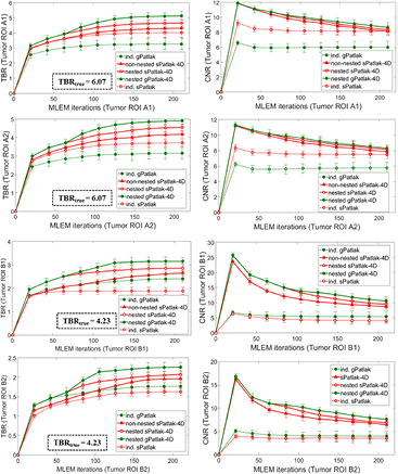
Figure 6. TBR (1st column) and CNR (2nd column) quantitative analysis for A1, A2, B1 and B2 target ROIs on simulated Ki parametric images for a range of indirect and direct (s/g)Patlak methods. The same number of nested Patlak ML-EM sub-iterations and gPatlak-4D initialization scheme are employed, as for figure 5. TBR and CNR scores were averaged over 20 noise realizations with the standard deviation illustrated with error bars.
Download figure:
Standard image High-resolution image3.1.3. sPatlak versus gPatlak 4D WB imaging.
A visual inspection of the ground truth Ki and kloss images and their comparison with the noise-free reconstructed Ki images in figure 5(a) (2nd row) suggests that, in general, the gPatlak indirect 3D and direct 4D methods were associated with more accurate Ki estimates than respective sPatlak methods. Furthermore, both noise-free and noisy gPatlak 4D reconstructions yielded relatively higher Ki TBR contrast scores, than respective sPatlak reconstruction, for tumor ROIs of group B, where a relatively higher degree of uptake reversibility (k4 = 0.012) was introduced in our simulations (table 1). Thus, our observations demonstrated the theoretical advantage of gPatlak over sPatlak algorithms, when evaluating regions exhibiting non-negligible uptake reversibility. However, the same results indicated lower Ki image noise for sPatlak versus the gPatlak 4 D methods. The respective noise-bias curves (figure 5(c)) confirmed the previous findings, as they revealed smaller bias at matched noise levels and higher noise at matched resolution (bias) for gPatlak 4D reconstruction methods.
Furthermore, in terms of lesion detectability performance, the results in figure 6 suggest that the main differences between sPatlak and gPatlak 4D methods were observed in TBR and CNR scores, with TBR being affected more profoundly. We attribute this finding to the relatively higher noise levels for gPatlak imaging, even within the 4D framework. Although bias and TBR contrast are enhanced with gPatlak 4D methods, the increased noise associated with gPatlak non-linear model eventually limits gPatlak 4D CNR scores. As a result, gPatlak 4D is not increasing the CNR scores as much as it enhances the TBR scores.
3.1.4. Conventional versus nested Patlak 4D ML-EM and number of nested sub-iterations.
The expected gain in ML-EM convergence rate for the nested relative to the conventional, i.e. non-nested, 4D sPatlak implementations was illustrated qualitatively and quantitatively in figures 5(b) and (c) respectively. In particular, visual inspection of B1 and B2 lesions contrast as a function of the iteration cycles in simulated Ki images of figure 5(b) suggested a faster contrast recovery, and thus convergence rate, for the nested sPatlak Ki images. In addition, the respective noise-bias curves in figure 5(c) indicated smaller bias values at matched noise levels for the nested sPatlak 4D implementation.
Moreover, a mildly faster 4D ML-EM convergence was recorded as the number of nested sub-iterations increased per global iteration step. This is conjectured from all three plots of the 2nd column of figure 7. However, the gain in bias and TBR contrast became progressively negligible when more than 20 sub-iterations were involved, as convergence had already been established at earlier iterations in these cases. Meanwhile, the noise was being steadily deteriorated in the same cases, due to the higher number of nested updates involved per global iteration step. As a result, for higher than 20 nested sub-iterations, image noise kept increasing relatively faster than TBR lesion contrast and, consequently, CNR started dropping at later iterations. Although not included in the results, it should be noted that a very small number of sub-iterations (<10) resulted in consistently slower convergence in all nested 4D algorithms.
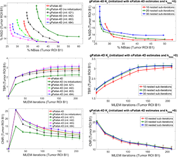
Figure 7. Ki noise-bias trade-off, TBR and CNR quantitative analysis over 20 noise realizations for simulated B1 ROI for different initialization schemes (1st column) and number of nested ML-EM Patlak sub-iterations (2nd column) for a range of conventional and novel 4D-Patlak methods. The sPatlak-4D and the first gPatlak-4D method (red and green curves at 1st column) were initialized with the conventional method (Ki = 1, kloss = 0, V = 1). All methods in 1st column utilized 20 sub-iterations. Finally, all gPatlak-4D methods of 2nd column were initialized with kloss = 0 and Ki and V values estimated from 63 sPatlak MLEM iterations.
Download figure:
Standard image High-resolution image3.1.5. Patlak 4D ML-EM initialization schemes.
The noise-free images in figure 5(a) demonstrate that the (s/g)Patlak 4D ML-EM algorithms converge in theory to the global optimal solution regardless of the initialization method. Thus, our findings indicated proper theoretical EM convergence properties for the implemented algorithms. In the presence of noise, however, the conventional method of initializing 4D ML-EM with Ki = 1, kloss = 0 and V = 1 parameter values, yielded correct EM convergence only in the case of 4D sPatlak method, as it can be conjectured by comparing 3rd and 4th row in figure 5(b). Nevertheless, as the Ki images of the last 2 rows in figure 5(b) illustrate, higher Ki lesion contrasts were attained with 4D gPatlak, compared to sPatlak (3rd row), after initializing the gPatlak 4D method with Ki and V estimates from the first 21 (5th row) or 3 × 21 = 63 (6th row) sPatlak iterations.
The importance of sPatlak-based initialization for gPatlak 4D algorithms was further demonstrated by the noted bias reduction as well as TBR and CNR score enhancements in figure 7 (1st column plots), when more sPatlak 4D global iterations were involved in the initialization of gPatlak 4D algorithm. However, after 3 cycles of 21 sPatlak ML-EM initial iterations, no additional benefit was observed for gPatlak 4D EM convergence rate. Thus, under noisy conditions, gPatlak 4D reconstruction may require a minimum number of sPatlak 4D iterations for its initialization, to ensure proper convergence and thus high quantification accuracy in Ki reconstructed images.
3.2. Clinical demonstration of feasibility and benefits of 4D WB Patlak imaging
In figure 8, we present a set of indirect and direct (s/g)Patlak Ki WB images from a patient dataset at a 10–45 min p.i. scan time window. Moreover, the respective SUV WB PET image is also shown, as acquired at 60 min p.i. with the standard-of-care static PET protocol. The directly reconstructed (s/g)Patlak WB Ki images were estimated after five cycles of 21 ML-EM global iterations each. A nested 4D ML-EM implementation was employed at each bed position involving 20 sub-iterations. Furthermore, the first 3 out of the 5 ML-EM iteration cycles of the gPatlak 4D WB reconstruction consisted of sPatlak 4 D ML-EM iterations to initialize the 4th cycle of gPatlak ML-EM iterations (figure 9).
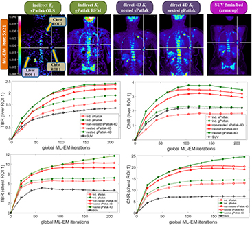
Figure 8. (1st row): clinical WB (s/g)Patlak Ki images, as estimated either indirectly or directly from the raw dynamic (10–45 min p.i) 18F-FDG PET data with 4D and indirect methods with patient arms at the bottom position to withstand longer scan duration. Also, the respective static SUV image obtained at 60 min p.i., after repositioning same patient with arms in the standard upper position (2nd and 3rd rows): TBR and CNR scores versus iterations for a range of (s/g)Patlak and SUV methods from a chest and a liver suspected tumor lesion ROIs.
Download figure:
Standard image High-resolution image
Figure 9. (1st row): clinical WB Ki images, estimated directly from the raw data of 6 WB passes with nested (s/g)Patlak 4D-MLEM methods. sPatlak 4D algorithm has been initialized with conventional method, while gPatlak 4D method utilizes the estimates of previous sPatlak 4D method after 3 cycles of 21 ML-EM iterations. All methods employ 20 nested sub-iterations. (2nd and 3rd rows): clinical TBR and CNR evaluation on 2 selected chest ROIs drawn from patient WB Ki images as a function of the initialization scheme and number of nested sub-iterations employed by the proposed (s/g)Patlak 4D WB reconstruction methods.
Download figure:
Standard image High-resolution image
3.2.1. Direct 4D Patlak versus SUV WB PET imaging in clinic.
The spatial noise levels visually observed in the background regions of the selected liver and chest target ROIs of WB 4D (s/g)Patlak Ki clinical images of figure 8 were comparable to the respective static SUV image noise. This is also evident by comparing the TBR and CNR scores of respective clinical Ki and SUV images for both evaluated ROIs in the same figure. In particular, the superiority of Ki imaging, relative to SUV, in terms of TBR contrast is also retained to nearly the same or higher degree in terms of CNR score. As CNR is derived from TBR after normalizing the latter with spatial noise in the target background, the previous observation suggest similar or lower quantitative levels of spatial noise between direct 4D Ki and SUV clinical images, at least for the two evaluated ROIs. Thus, our results demonstrate the clinical feasibility of 4D WB Patlak Ki methods, when applied on a streamlined 6-pass WB PET protocol. In addition, the superior TBR and CNR 4D Ki scores, relative to SUV, on the two identified ROIs indicate potential enhancement of tumor detectability performance, when complementing the currently established in clinic WB SUV imaging protocols with the proposed direct 4 D WB (s/g)Patlak methods.
3.2.2. Direct 4D versus indirect Patlak WB clinical imaging.
The images in figure 8 illustrated the lower noise of direct 4D relative to indirect Patlak methods. Moreover, the quantitative plots in figure 8 demonstrated the superior TBR and CNR performance for all 4D Patlak methods, compared to the respective indirect methods, particularly for the chest ROI. The improvement was more evident in terms of the CNR metric, owing to the lower noise levels observed in the 4D reconstructions versus indirect Patlak analysis. Our clinical findings confirmed the simulation results and can be explained by the more efficient utilization of the acquired data with 4D Patlak algorithms. Finally, the quantitative TBR and CNR analysis suggested that the gain observed when switching from indirect to direct 4D Patlak methods is relatively larger than the respective gain between standard and generalized Patlak models.
3.2.3. sPatlak versus gPatlak 4D WB clinical imaging.
Our clinical validation results in figure 8 demonstrated the superior TBR lesion contrast scores for nested gPatlak 4D Ki images, both via the qualitative inspection of the respective patient WB Ki images as well as through the quantitative TBR analysis in both evaluated ROIs. Moreover, despite the higher noise levels observed in gPatlak Ki images, relative to sPatlak, the highest clinical ROI CNR scores were systematically observed for the former. Besides, the clinical TBR and CNR score differences between the two 4D Patlak methods were not as significant as the respective differences between (i) indirect sPatlak and gPatlak or (ii) direct versus indirect Patlak methods. In other words, the differences between the two Patlak models were less significant in the 4D framework.
3.2.4. Clinical impact of number of nested sub-iterations and gPatlak initialization.
The series of WB Ki images in figure 9 illustrate the convergence of sPatlak and gPatlak 4D methods, when applied to the same patient dataset and after being initialized with the proposed schemes. The two 4D algorithms converged to different but similar sPatlak and gPatlak solutions in the last two cycles of 21 iterations.
Moreover, the TBR and CNR plots describe the quantitative effect on 2 chest ROIs of the number of nested ML-EM sub-iterations as well as that of sPatlak-based initialization for gPatlak 4D algorithm. In particular, the plots of the 2nd row suggested superior TBR and CNR performance for both ROIs in clinical gPatlak-4D Ki images, when at least 3 × 21 ML-EM sPatlak iterations are employed for its initialization. Any higher number of iterations only resulted in negligible convergence acceleration. Furthermore, the TBR and CNR scores of the 3rd row suggested a minimum number of 20 nested ML-EM sub-iterations to sufficiently accelerate convergence without increasing noise in the Ki images.
4. Discussion
4.1. Benefits, limitations and respective solutions for nested 4D (s/g)Patlak WB ML-EM algorithms
Initially, our evaluation concentrated on the benefits of direct 4D versus indirect sPatlak WB imaging. The simulation results illustrated considerable noise reduction at matched bias in Ki images when 4D reconstruction was employed, especially for regions of low uptake signal and therefore high noise. Moreover, the respective clinical evaluation on clinical data revealed improved CNR Ki scores at matched contrast in suspected tumor regions for the 4D methods. Nevertheless, a known limitation for 4D parametric reconstruction algorithms is the slower convergence rate compared to the indirect methods, thus constraining their clinical adoption. Therefore, we suggested exploiting the optimization transfer principle to enable convergence acceleration via a nested ML-EM implementation framework. By nesting multiple image-based ML-EM Patlak parameter updates within each slower tomographic ML-EM iteration step, we allowed for a larger number of Patlak parameter updates per global iteration at a negligible added computational cost and thus effectively accelerated the convergence.
Subsequently, the study focused on 4D reconstruction performance assessment between sPatlak and gPatlak ML-EM methods with the simulation results indicating reduction in Ki bias for gPatlak at matched noise levels. The comparative evaluation on WB Ki patient images also suggested superior CNR scores at matched number of iterations. However, gPatlak 4D method assumes a non-linear model for the relationship between the final parameter estimates and the dynamic data. Our proposed nested ML-EM implementation overcame this issue by targeting the iterative estimation of the overall gPatlak response function, instead of the individual gPatlak parameters, as only the former is linearly related with the dynamic image estimates. Then, a nested ML-EM implementation similar to sPatlak 4D method was made possible. Eventually the individual gPatlak parameters were estimated analytically at the end of the last nested sub-iteration from the last response vector estimate. Besides, the ML-EM estimated response vector and not the gPatlak parameters were being used in the next global iteration. Thus, the designed algorithm fully retains the ML-EM properties to ensure KL distance minimization between the data and the estimates and, thus, its theoretical EM convergence to a global ML solution (Barrett and Myers 2004). Indeed, our evaluation on both simulated and clinical data revealed a faster convergence for the nested 4D (s/g)Patlak algorithms, thus demonstrating their higher clinical adoptability.
Nevertheless, the gPatlak 4D ML-EM optimization becomes more susceptible to data noise, as now the number of the response vector elements to be estimated is considerably high. On the other hand, the sPatlak 4D algorithm, although relatively less quantitative than gPatlak, is more robust to noise, as it optimizes a log-likelihood function with respect to just two parameters: Ki and V. Therefore, we proposed initializing the gPatlak 4D algorithm with estimates derived after a few sPatlak 4D ML-EM iterations and zero kloss. Indeed, both the simulated and clinical results showed incomplete gPatlak 4D convergence, unless the suggested sPatlak-based initialization scheme was applied.
Although our simulation and clinical findings have confirmed the theoretical expectations, we recognize the clinical value of expanding current validation study to a larger cohort of patients to involve a wider range of tracer kinetics and commercial scanner acquisition and reconstruction technologies. In fact, we are currently conducting a systematic assessment of TOF and resolution modeling techniques on direct 4D and indirect WB (s/g)Patlak imaging methods (Karakatsanis et al 2014b, 2015c).
4.2. Complementing conventional 3D SUV with 4D Patlak PET image reconstruction
Static 3D PET imaging utilizes the clinically established SUV metric to estimate a temporal instantiation of the tracer dynamic distribution, as integrated over a time frame, normalized to injected dosage and lean body mass (Wahl and Buchanan 2002). Nevertheless, SUV is considered semi-quantitative, as it is dependent of the acquisition time window and the metabolic and dietary condition of the subject (Keyes 1995, Huang 2000, Thie 2004, Boellaard 2011, Durand and Besson 2015).
On the contrary, dynamic PET imaging can track the signal distribution over space and time, thus enabling imaging of parameters describing the physiological in vivo uptake of the administered tracer. By correlating the measured tissue TACs with the blood input function, graphical analysis methods enable quantitative image-based assessments that may be substantially less dependent on the acquisition time window and the current metabolic state of the subject. As a result, 4D imaging may facilitate more objective evaluations between imaging studies of the same subject, thus paving the way for enhanced quantification in treatment response monitoring and image-guided diagnostic and therapeutic schemes.
Therefore, in this study we view the proposed 4D (s/g)Patlak reconstruction framework mainly as a quantitative complement to the standard-of-care single-pass 3D PET SUV protocols. The presented 4D imaging methods could constitute the early phase (0–40 min p.i.) followed by the conventional SUV PET scan (60–80 min p.i.). Alternatively, dynamic WB PET acquisition could instead be delayed towards the more standard post-60 min windows and eventually replace single-pass WB SUV with a multi-pass WB scan. Then, the SUV metric would be estimated by properly adding together the dynamic PET frames of each bed across time, while the (s/g)Patlak Ki metrics would be derived from 4D (s/g)Patlak reconstructions of the same data. Although, this approach would alleviate the need for 2 anatomical scans, thus permitting its application within a PET/CT framework too, it would also require inference of the missing early section of the input function (Zhou et al 2012, Karakatsanis et al 2015d). This method has been evaluated in a combined SUV/Patlak clinical study (Karakatsanis et al 2015b).
4.3. Application scope of 4D generalized Patlak imaging
In this study, the presented 4D (s/g)Patlak methods have been designed and evaluated for multi-bed or WB acquisitions to demonstrate their clinical potential in oncology, where large axial FOVs are important for assessing potential metastatic tumors. Nevertheless, the proposed methods can be also utilized in more specific clinical applications involving single-bed FOVs, such as cardiovascular, neurologic or specific tumor type evaluation studies (Dimitrakopoulou-Strauss et al 2002, Sanz and Fayad 2008, Oo et al 2013).
We laid emphasis on Ki image evaluation, as this parameter has been found to correlate well with SUV metric over patient population (Freedman et al 2003). The Ki parameter reflects a principal kinetic component that conveniently summarizes a major portion of the clinically relevant information contained in 4D FDG PET data. Nevertheless, we have also demonstrated the importance of the kloss parameter as well, in terms of Ki quantification and TBR. Furthermore, we observed that kloss and V images correlated well with the respective ground truth values, although their robustness was found lower than that of Ki and dependent on noise and  inversion accuracy. Despite our focus on Ki quantification, we acknowledge the clinical potential of kloss and V imaging, especially when correlated with Ki and SUV metrics, and we plan investigating their clinical relevance in oncology and other disease mechanisms.
In addition, although this study has been focusing on 18F-FDG tracer, as this is the most widely used PET radiotracer in oncology (Phelps et al 1979, Hustinx et al 2002), it could be also well applied to other radiotracers of similar half-lives, such as 18F-FLT (Been et al 2004), 18F-FMISO (Thorwarth et al 2005), and 18F-NaF (Siddique et al 2011), utilizing equivalent protocols. Moreover, the support for gPatlak model may enable robust kinetic analysis for a range of tracers with varying degree of uptake reversibility in different tissues, thus widening the application scope. Finally, all presented algorithms have been implemented within the open-source STIR platform for a broader utilization by the research community.
4.4. Data utilization efficiency and noise characterization between 4D and indirect Patlak imaging
In the direct 4D parametric PET image reconstruction framework, the complete 4D measurements space is directly related with the kinetic parameters image space through a 4D system response model. As a result, 4D algorithms directly exploit measurements from all dynamic sinograms. On the contrary, indirect parametric imaging employs frame-by-frame 3D reconstructions only utilizing the counts from a single sinogram each time. As the latter approach exploits measurements from a smaller pool of data, it will inevitably result in higher noise levels that are subsequently propagated in the final Patlak images through the post-reconstruction statistical regression estimation process. Therefore, parametric image noise is expected to be lower with direct 4D algorithms, thanks to the more efficient utilization of the measured counts (Barrett et al 1994, Reader et al 2006). In addition, this difference becomes more apparent for 4D PET data of low count statistics (Reader and Verhaeghe 2014), such as in the case of dosage minimization (Karakatsanis et al 2014e) or WB dynamic acquisition protocols.
Indirect Patlak regression is conducted on the reconstructed images where the statistical noise is spatially correlated and unknown, as it depends on numerous factors, including number of iterations, resolution modeling kernel and object shape (Barrett et al 1994, Rahmim et al 2013, Rahmim and Tang 2013, Ashrafinia et al 2014). Consequently, noise distribution in the image space is often approximated, thus increasing the likelihood for noise-induced bias in the estimates (Reader and Verhaeghe 2014). On the contrary, direct 4D reconstruction is applied on the raw measurements space, where the noise can be accurately described, as it follows the well-known Poisson distribution. This property facilitates robustness especially for non-linear algorithms, such as the gPatlak 4D method, thus closing the gap between linear and non-linear performance in terms of noise-induced bias. Indeed, our results indicated smaller differences between the two Patlak methods in the direct 4D relative to the indirect framework.
5. Conclusions
In this study, we designed and implemented a set of linear and non-linear 4D (s/g)Patlak reconstruction methods capable of estimating parametric images directly from single- or multi-bed dynamic PET sinogram data. Standard as well as novel generalized Patlak models were integrated within the 4D ML-EM reconstruction framework to support a wider range of PET tracer kinetics with or without uptake reversibility. The direct 4D Patlak algorithms always outperformed the respective indirect methods in terms of noise at matched resolution levels and CNR at matched contrast. The observed noise reduction between indirect and 4D imaging was more profound in the case of the non-linear gPatlak model. In addition, gPatlak 4D imaging outperformed the respective sPatlak analysis for both simulated and clinical data in terms of contrast at matched noise scores and matched number of iterations. Moreover, the presented direct reconstruction algorithms utilized the optimization transfer principle to efficiently nest the faster Patlak iterative ML-EM update process within each global ML-EM iteration step and thus accelerate EM convergence rate for enhanced clinical adoption of the presented methods.
To conclude, we demonstrated the clinical feasibility and quantitative benefits of complementing standard-of-care WB SUV imaging with the proposed 4D WB (s/g)Patlak reconstruction framework. The additional surrogate metrics offered by the presented family of 4D Patlak graphical analysis methods, such as the tracer net uptake rate constant Ki and net efflux rate constant kloss, could extend quantification capabilities beyond the currently established SUV metric. In addition, the proposed 4D methods is associated with relatively low noise levels, comparable to static SUV images and supports a wide range of tracer kinetics including uptake reversibility. Moreover, the 4D (s/g)Patlak framework was supported with advanced optimization transfer and initialization schemes to ensure proper and faster 4D EM convergence rates and, thus, further facilitate clinical adoption. Furthermore, all introduced 4D Patlak reconstruction algorithms have been implemented in open-source STIR platform to enable their broader utilization by the research community for further developments towards quantitative PET. Therefore, the presented 4D PET reconstruction methods in this study have been designed and implemented such that they can efficiently, robustly and easily be translated to the clinic, to enhance quantification in existing routine PET protocols for improved diagnostic and theranostic applications in molecular imaging.
Acknowledgments
The authors would like to thank Drs Kris Thielemans and Charalampos Tsoumpas for their feedback regarding the software versioning and control procedures to facilitate integration of our developments into the STIR package. This work was supported by the Swiss National Science Foundation under Grant SNSF 31003A-149957, Siemens Medical Solutions and the NIH grant 1S10RR023623.