
Abstract
A computer model of a patient-specific clinical 177Lu-DOTATATE therapy dosimetry system is constructed and used for investigating the variability of renal absorbed dose and biologically effective dose (BED) estimates. As patient models, three anthropomorphic computer phantoms coupled to a pharmacokinetic model of 177Lu-DOTATATE are used. Aspects included in the dosimetry-process model are the gamma-camera calibration via measurement of the system sensitivity, selection of imaging time points, generation of mass-density maps from CT, SPECT imaging, volume-of-interest delineation, calculation of absorbed-dose rate via a combination of local energy deposition for electrons and Monte Carlo simulations of photons, curve fitting and integration to absorbed dose and BED. By introducing variabilities in these steps the combined uncertainty in the output quantity is determined. The importance of different sources of uncertainty is assessed by observing the decrease in standard deviation when removing a particular source. The obtained absorbed dose and BED standard deviations are approximately 6% and slightly higher if considering the root mean square error. The most important sources of variability are the compensation for partial volume effects via a recovery coefficient and the gamma-camera calibration via the system sensitivity.
Export citation and abstract BibTeX RIS

Content from this work may be used under the terms of the Creative Commons Attribution 3.0 licence. Any further distribution of this work must maintain attribution to the author(s) and the title of the work, journal citation and DOI.
For more information on this article, see medicalphysicsweb.org
1. Introduction
One increasingly used form of radionuclide therapy (RNT) is peptide receptor radionuclide therapy (PRRT), one example being 177Lu-DOTATATE used for treatment of disseminated neuroendocrine tumours. These treatments are associated with renal and haematological toxicity (Kwekkeboom et al 2005, Bodei et al 2008, 2015), thereby limiting the activity that can be administered. One strategy to limit toxicity while still being able to maximize the administered activity is to perform patient-specific dosimetry, i.e. determination of the absorbed dose to the critical organs. The radionuclide 177Lu, is a beta emitter that also emits gamma photons, allowing for gamma-camera imaging and image-based renal dosimetry, either with planar images or with single photon emission computed tomography (SPECT) (Garkavij et al 2010).
An increasing amount of evidence is emerging of dose-effect relationships in RNT (Strigari et al 2014), but historically it has been considered difficult to establish such connections. Complicating factors in such investigations have been possibly large, but seldom reported, uncertainties in the estimated absorbed dose and radiobiological considerations, such as effects of the patient-specific pharmacokinetics on the absorbed-dose rate and thereby on the relative effect per unit of absorbed dose (Barone et al 2005). As a consequence of the latter, the concept of biologically effective dose (BED) has gained interest within RNT due to its theoretical potential to account for different irradiation time-patterns.
Investigation of uncertainties in quantitative nuclear-medicine tomographic imaging has a history involving works by e.g. Budinger et al (1978) and Carson et al (1993). More recently, precision and accuracy has been investigated by e.g. Shcherbinin et al (2008) and Zeintl et al (2010), and the specific aspect of gamma-camera calibration has been studied by e.g. Anizan et al (2014) and Anizan et al (2015). Recent studies have often used anthropomorphic computer phantoms, e.g. the XCAT phantom (Segars et al 2010). This phantom type has been used for e.g. estimation of the precision and accuracy of activity quantification and residence time for different anatomy configurations (He et al 2009) and of effects of organ delineation (He and Frey 2010). An alternative to tomographic imaging is to use planar gamma-camera imaging, for which uncertainties in activity quantification have also been analysed (Norrgren et al 2003). However, for renal dosimetry in 177Lu-PRRT, planar-based quantification suffers from problems caused by activity in the intestines being superpositioned on the kidneys in the images (Garkavij et al 2010). Internal dosimetry can be considered a multi-step process with an uncertainty associated with each step (Stabin 2008). The majority of studies on uncertainty have focused on one or a few steps, but, to the best of our knowledge, no study has yet investigated the propagation of uncertainty through the complete process to a combined uncertainty in absorbed dose or BED.
One particular problem when discussing absorbed dose in RNT is the heterogeneous distribution of the radiopharmaceutical within organs. Depending on the range of the particles emitted by the radionuclide, this may also translate into an heterogeneous small scale absorbed-dose distribution (de Jong et al 2004, Konijnenberg et al 2007). Thus, any statement of the absorbed dose has to be associated with a specification of the structure to which the absorbed dose has been estimated, be this the mean absorbed dose to an entire organ or the mean absorbed dose to substructures within that organ. In the context of 177Lu-PRRT, structures for which absorbed-dose estimates are of particular interest may be the whole kidney, the renal cortex and medulla, or the most radiosensitive structures glomeruli and tubules (Fajardo et al 2001). In this work, the measureand (the quantity intended to be measured) will be defined as the mean absorbed dose to the renal cortex and medulla, i.e. the mean absorbed dose on an organ level but excluding the renal pelvis.
Extending dosimetry to cover BED, the uncertainty in this value is also relevant. However, since the BED is a model-based concept rather than a real physical quantity some care has to be observed with regards to the meaning of such an uncertainty. Also, considerable uncertainties in radiobiological parameters such as the  -ratio and the repair half-times have been reported (Bentzen and Joiner 2009), making the connection between patient measurements and BED uncertainty less direct. Nevertheless, it is not obvious that an uncertainty in absorbed dose directly translates into a given uncertainty contribution to BED, since the latter is not only dependent on the absorbed dose, but also on the shape of the absorbed-dose rate function.
Guidelines for the reporting of measurement uncertainties have been presented in the Guide to the expression of uncertainty in measurement (GUM) (JCGM 2008a). The traditional way of evaluating the uncertainty associated with the output quantity in an expression involving one or several input quantities is to use the law of propagation of uncertainty. This law analytically propagates the standard uncertainties associated with involved variables to a combined standard uncertainty for the output quantity. A standard uncertainty is interpreted as the standard deviation (SD) of the probability distribution of the variable concerned. An alternative is to use a Monte Carlo (MC) method, as summarized in a supplement to the GUM (JCGM 2008b). The principle is here to propagate the probability distributions of input variables through the measurement model, instead of only its first and second moments.
The aim of this work is to examine the measurement uncertainty of renal absorbed dose in SPECT/CT-based dosimetry for 177Lu-DOTATATE using an MC approach. The MC analysis propagates uncertainties through the dosimetry process, starting from uncertainty in gamma-camera calibration, ending at the SD and root mean square error (RMSE) in kidney absorbed dose and BED (excluding variability in radiobiological parameters). As basic tools, MC simulation of gamma-camera imaging (Ljungberg and Strand 1989) and three patient models, as constituted by anthropomorphic computer phantoms coupled to a pharmacokinetic model of 177Lu-DOTATATE (Brolin et al 2015), are used.
2. Material and methods
In this section the clinical dosimetry process is first described, followed by its model counterpart.
2.1. Clinical dosimetry process
2.1.1. Gamma-camera calibration.
The calibration factor for conversion of the detected count rate in the gamma camera images to activity is determined by measuring the system sensitivity, i.e. the count rate per unit of activity in air (Ljungberg et al 2003). This is done by planar imaging of Petri dishes with thin layers of activity. The activity solution is prepared in a vial, where the activity concentration is determined using a scale and a radionuclide calibrator (Fidelis, Southern Scientific, Henfield, UK). The activity is dispensed into the three Petri dishes, which are individually imaged for the two camera heads. For analysis of the count rate, a circular region of interest (ROI) is defined with a radius 2 cm larger than the source radius, to account for resolution-induced spill-out, and the system sensitivity is determined from the number of counts in the ROI. The average from the three Petri dishes is used as the sensitivity.
2.1.2. CT-derived density images.
In the methods used for attenuation and scatter corrections within the tomographic reconstruction (section 2.1.3), and for calculation of the absorbed-dose rate from the SPECT images (section 2.1.5), images of the mass-density distribution in the patient are required. In connection with SPECT imaging, computed tomography (CT) images are acquired using a low-dose protocol, employing a tube voltage of 120 kV. The CT image Hounsfield numbers (HN) are then converted off-line to mass densities using a calibration-based relationship. This relationship is obtained from previous measurement of a commercial CT calibration phantom with inserts of known densities (CIRS, Norfolk, VA, USA), using the same settings as for patient measurements (Sjögreen et al 2002, Sjögreen-Gleisner et al 2009, Garkavij et al 2010). Details of this calibration are described in section 2.3.2.
2.1.3. SPECT imaging.
The patient is infused with 7400 MBq 177Lu-DOTATATE over 30 min and is imaged using SPECT at nominally 0.5 h, 24 h, 96 h and 168 h post end of infusion (p.i.). The gamma camera is a GE Discovery 670 (GE Healthcare) equipped with medium energy general-purpose collimators, and acquisition employing a 15% energy window centred at 208 keV, 60 projections in full rotation mode and a  matrix with a pixel size of
  mm2. The time per projection is 45 s, making the total imaging time approximately 22.5 min. Quantitative image reconstruction is performed using ordered subset expectation maximization (OS-EM) with eight iterations and ten subsets employing compensation for attenuation, scatter (effective scatter source estimation) and distance dependent resolution (Frey and Tsui 1996, Kadrmas et al 1998). The CT-derived density image is used for attenuation and scatter corrections in the reconstruction, and is for that purpose recalculated to attenuation coefficients by multiplication to the mass-attenuation coefficient for 208 keV for soft tissue and bone, for low- and high density regions, respectively.
2.1.4. Volume of interest delineation.
Volumes of interest (VOIs) including the renal cortex and medulla but excluding the renal pelvis are manually outlined on the SPECT/CT images, using mainly the CT information for guidance. Each kidney and imaging time-point is considered separately.
2.1.5. Calculation of renal absorbed-dose rate.
In the calculation of energy deposition from the SPECT estimated activity distribution, electrons and photons are handled separately. Because the mean range of the electrons is considerably smaller than the spatial resolution of the SPECT system, the electron energy is assumed to be absorbed locally in each voxel. Thus, the electron absorbed-dose rate is assumed to be proportional to the voxel activity, and is calculated by multiplication to the emitted electron energy per decay, and division by the voxel mass as determined from the mass-density image (Sjögreen-Gleisner et al 2009, Ljungberg and Sjögreen-Gleisner 2011). The absorbed-dose rate from photons is obtained via an MC simulation program for calculation of absorbed dose from images (Ljungberg et al 2003). The SPECT-derived activity image is here used as source map, and the CT-derived density image is used to derive maps of interaction probabilities, and for estimation of the voxel mass. The emission spectrum for 177Lu is retrieved from the NuDat 2 database (National Nuclear Data Center 2014). Nine million histories are simulated for each imaging time-point.
VOIs are applied to each of the absorbed-dose rate maps and the mean VOI values calculated. Partial volume correction is then applied to compensate for the net spill-out of counts caused by limited spatial resolution, which would otherwise yield an underestimation of the activity concentration and thus absorbed-dose rate. The partial volume correction is applied to the mean electron absorbed-dose rate only, using a fixed recovery coefficient (RC) of 0.84. Since the electron absorbed-dose rate is assumed to be proportional to the activity concentration, partial volume correction is considered necessary. Photons, on the other hand, have a non-negligible mean-free path compared with the spatial resolution of SPECT imaging, and effects of resolution are considered to be less important. Thus, the mean VOI values for electrons (divided by the RC) and photons are added and taken as representative for the cortex and medulla of each kidney. The value of the RC was estimated in a separate sub-study (Mortensen et al 2014) where technologists delineated kidneys in MC simulated 177Lu PRRT images, as further described in section 2.3.4.
2.1.6. Calculation of absorbed dose and BED.
Typical sets of time-dose rate data for patients do not show a consistent mono-exponential pattern due to an unpredictable behaviour of the 0.5 h measurement, which, in turn, is related to the initial phase of excretion of 177Lu-DOTATATE through the kidneys. To avoid this first data point affecting the extrapolation of the absorbed-dose rate curve beyond the last time-point, a simplistic approach is assumed for the initial part of the time-activity curve. Thus a fitting function with an initial linear part and a tailing exponential part is used. The exponential function is fitted to the three last points using non-linear least squares, while the linear part is calculated from the first data point and the value of the exponential function at the second time-point. The linear function is also used for extrapolation back to time zero. The absorbed dose is obtained by analytic integration of the absorbed-dose rate function from zero to infinity.
The BED is calculated using discrete convolution (Gustafsson et al 2013) between the fitted absorbed-dose rate function and a mono-exponential repair function with a repair half-time of 2.8 h using an  -ratio of 2.6 Gy (Thames et al 1988).
2.2. Phantoms
2.2.1. Anthropomorphic computer phantoms.
Three voxel phantoms with different body constitutions from the XCAT family (Segars et al 2010, 2013) coupled to a pharmacokinetic model of 177Lu-DOTATATE were used. As described by Brolin et al (2015), each phantom structure follows a well-defined time curve of activity and absorbed-dose rate as a function of time. Because the arms of the original phantoms introduced an unrealistic camera-rotation radius for SPECT imaging simulations they were omitted from this work, while preserving the activity concentrations of each phantom structure. An illustration of the anatomies of the three computer phantoms is shown in figure 1. General properties of these phantoms are given in Brolin et al (2015) and some properties of the kidney anatomies are given in table 1.

Figure 1. Total intensity projections of the mass-density distributions of the three phantoms (upper panel) and SPECT images at 1 d p.i. (lower panel).
Download figure:
Standard image High-resolution imageTable 1. Masses in gram of the kidney structures cortex, medulla and pelvis for the three different phantoms.
| Phantom number | Left cortex | Right cortex | Left medulla | Right medulla | Left pelvis | Right pelvis |
|---|---|---|---|---|---|---|
| 1 | 107 | 117 | 43 | 36 | 8 | 6 |
| 2 | 167 | 136 | 75 | 46 | 12 | 10 |
| 3 | 116 | 93 | 49 | 49 | 5 | 7 |
The absorbed-dose rate curves of the phantom kidneys can be considered as reference curves to which estimated absorbed dose-rate curves, and their integration to absorbed dose, can be compared. In addition to kidney absorbed doses, the reference absorbed-dose rate curves also allow for calculation of reference BED values using discrete convolution (Gustafsson et al 2013). The reference BED was calculated under the same assumptions of radiobiological parameters as for the clinical procedure (section 2.1.6).
2.2.2. Physical phantom.
For benchmarking of the results obtained with the simulation process, an experiment was conducted using a physical anthropomorphic phantom (Heart/Thorax phantom, Radiology Support Devices Inc., Long Beach, CA, USA). The phantom liver insert was filled with an activity concentration (with respect to mass) of approximately 0.5 MBq g−1 177Lu-DOTATATE in water, which was prepared using a radionuclide calibrator and a scale. The background was filled with water and SPECT/CT imaging was performed on seven occasions, between one and nine days after filling, using the same camera system and acquisition settings as described for the patient procedure. The reason for using the comparably large liver insert was that it was difficult to find an object with an activity distribution which resembled that of kidneys, where the kidney RC used for the clinical dosimetry was applicable. Thus, the uncertainty introduced by the compensation for partial volume effects was not addressed in this experiment. The reference value of the cumulated activity concentration was obtained as the integral from 0 to infinity of the activity concentration via the initial liver activity concentration and the physical half-life of 177Lu. Figure 2 shows images of the physical phantom.
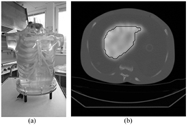
Figure 2. (a) The physical phantom. (b) An example of a SPECT/CT image 6 d after filling also showing the VOI used for evaluation of liver activity concentration.
Download figure:
Standard image High-resolution image2.3. Dosimetry process model
An overview of the dosimetry process model, including sources of uncertainty, is shown in figure 3. The process illustrated in this figure will henceforth be referred to as the MC pipeline.
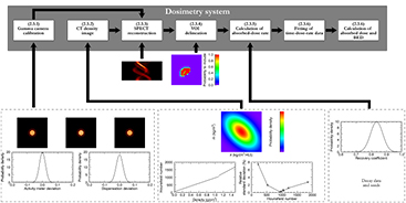
Figure 3. The dosimetry process model. The system is considered as a series of modules each processing the input of previous modules and possibly adding uncertainties. The numbers in the upper panel boxes refer to the subsections in section 2.3.
Download figure:
Standard image High-resolution image2.3.1. Gamma-camera calibration.
The measurement of the gamma-camera sensitivity was modelled by simulating a low-noise projection of a thin circular disk of 177Lu 10 cm in diameter, using the SIMIND MC program (Ljungberg and Strand 1989).
Images corresponding to realistic activities and measurement times were obtained by rescaling the projection image. Nominally, an activity of 15 MBq and a total measurement time of 10 min were assumed. Uncertainty in the activity actually contained in the Petri dish was modelled by adding two Gaussian random numbers, where the first accounted for uncertainty in the activity meter, while the second was mainly related to dispensation. After rescaling images to the resulting activity and measurement time, Poisson-distributed noise was added by replacing the projection pixel values with random numbers following Poisson distributions having expectation values equal to the values of the rescaled image.
The relative SD of the measurement of 177Lu in the activity meter (2%) was determined from the uncertainty of the calibration factor for 177Lu combined with an uncertainty estimated from weekly measurement of standard calibration sources. The relative SD associated with the Gaussian affecting each Petri-dish individually (2.2%) was estimated by reviewing the repeatability of our gamma camera, correcting for the variance caused by Poisson noise in the images.
Analysis of the resulting images was performed using the procedure described in section 2.1.1. The sensitivity was estimated as the number of counts in this ROI divided by the product of the nominal activity (i.e. 15 MBq) and the measurement time.
This process was repeated three times to mimic the three Petri dishes used in practice. The uncertainty in the activity meter measurement affected all three repetitions equally, since this effect is likely to be the same for all three dishes, while the second source of uncertainty, mainly related to dispensation, was individually sampled for each dish. The resulting camera sensitivity was calculated as the average of the three measurements.
2.3.2. CT-derived density images.
From the anthropomorphic phantoms, co-aligned density images were obtained in the same voxel size as the SPECT images. In order to mimic the real situation, where acquired CT images are converted to mass-density distributions, a two-step process was followed. To mimic the variability in CT-image values due to different patient configurations, experiments were conducted by imaging the CT calibration phantom using the same settings as for patient acquisitions. Layers of water-equivalent material were added to the phantom surface, thus varying the total thicknesses between 27 cm and 39 cm in the anterior-posterior direction. In the CT-images, VOIs were drawn in the density inserts of the phantom, and the mean and SD in HN for the VOIs were recorded, thus capturing the variability due to different thicknesses. For densities in between those of the phantom inserts SDs were obtained by linear interpolation of the experimentally obtained values. Mean values were interpolated by fitting a two-segment piecewise linear function to the HN-versus-density data using least squares. This function form was used to approximate the higher mass-attenuation coefficient of cortical bone as compared to soft tissue. The breakpoint between the two linear segments was set to 1.1 g cm−3. The inversion of this function was used as the calibration curve from HN to density, calculating the HN breakpoint (i.e. the HN corresponding to the destiny breakpoint) from the high density linear segment.
2.3.2.1. Model implementation.
To simulate CT images, the densities as defined for the anthropomorphic phantoms were converted to HN using the experimentally obtained piecewise linear relationship. To introduce uncertainty in these simulated CT images, corresponding to the variability in HN obtained for different patient configurations, the HN in each of the phantom structures (i.e. on a structure rather than voxel basis) was perturbed by a random number sampled from Gaussian distributions with the experimentally determined SDs in HN. Further, to mimic uncertainties introduced in the conversion of HN to densities, the covariance matrices of the inverted piecewise linear curve parameters were used to derive a new, perturbed, HN-versus-density calibration function, assuming multivariate Gaussian distributions for the parameters of each linear segment in the curve. This perturbed calibration function was then used for converting the simulated CT images back to densities.
2.3.3. SPECT imaging.
Each of the phantom structures was individually processed using SIMIND (Ljungberg and Strand 1989), producing essentially noise-free structure projection images. Full projections were generated by combining the organ projections for which the pixel values were first scaled according to the activity of each structure at a specific time-point. The activity in each organ was derived from the time-activity curves of the pharmacokinetic model, assuming a total activity of 7400 MBq at start of infusion. Instead of assuming a static activity distribution over the SPECT acquisitions, the activity values were sampled at the time of each projection. Sixty projections were simulated, each with an acquisition time of 45 s, giving a total time of 22.5 min.
The SPECT imaging start time-points were not kept fixed at their nominal values. In order to estimate clinically realistic distributions of imaging start time-points, data from a hybrid planar SPECT/CT dosimetry scheme currently used at our institution were used. The data consisted of imaging start time-points in 66 patient time series. The mean (SD) for the different imaging time-points were 0.4 h (0.1 h), 21.3 h (1.4 h), 93.3 h (1.8 h) and 165.8 h (2.1 h) p.i. For the last time point, three of the 66 cases were excluded since these were acquired on a different day than the seventh day p.i. In the MC pipeline, the imaging time-points were sampled as independent variables from linearly interpolated versions of the empirical distributions. The resulting SPECT projection images were corrupted with Poisson distributed noise. Tomographic reconstruction was performed as in the clinical procedure (section 2.1.3).
2.3.4. VOI delineation.
The operator-dependence in the delineation of renal VOIs in SPECT/CT images was analysed in a previous study (Mortensen et al 2014). In that study three experienced technologists delineated renal VOIs in both patient SPECT/CT images and in the simulated SPECT/CT images, thus giving an estimate of the VOI delineation contribution to bias and imprecision of renal absorbed doses. In the current study, the technologists' VOIs, three for each kidney of each anthropomorphic computer phantom, were used to derive maps of the probability that a particular voxel was included in a renal VOI. The probability for voxel inclusion was estimated as the fraction of operators including that voxel, i.e. 0,  ,
,  , or 1, which were used as basis for the random variation of VOIs in the MC pipeline. Since the technologists' delineation was mainly performed using the CT for guidance, one probability map per phantom kidney was used for all imaging time-points.
2.3.5. Calculation of renal absorbed-dose rate.
The simulated SPECT images were processed according to the clinical procedure (section 2.1.5).
Uncertainty in the emitted energy in the decay of 177Lu was modelled in this step. The 177Lu radionuclide data used for the clinical procedure were taken as a starting point, but the yields and energies of photons and electrons were sampled from Gaussian distributions with standard deviations according to the standard uncertainty given in the NuDat2 database (National Nuclear Data Center 2014).
Uncertainty in the RC, used for correction of the electron absorbed-dose rate, was modelled as a Gaussian distribution with an expectation of 0.84 and an SD of 0.04, independent of kidney size and kidney-to-background ratio. This choice of RC (mean and SD) was based on the results of the technologists' work described above.
2.3.6. Calculation of absorbed dose and BED.
The absorbed dose and BED were calculated as described in section 2.1.6.
2.4. Application of the dosimetry process model
2.4.1. Full model.
The full dosimetry process model was applied for all three phantoms and the absorbed dose and BED to left and right kidney were estimated in 256 realizations. To investigate possible systematic deviations in the absorbed-dose estimate for the particular kidney the mean absorbed dose and BED were calculated and compared to their reference values, while the dispersion around the mean was quantified as the SD. The combined result of systematic effects and dispersion was described using the RMSE.
2.4.1.1. Reduced models.
To investigate the decrease in kidney absorbed-dose dispersion when removing sources of uncertainty from the dosimetry process, each of the contributing sources were one by one kept fixed. These reduced models were investigated for the left kidney of phantom 1 only, by excluding variability in the (a) RC only; (b) gamma-camera sensitivity; (c) VOI delineation; (d) 177Lu radionuclide data; (e) density map generation; (f) imaging time point, and (g) noise in the SPECT projections. For all cases, i.e. also including cases (b)–(f) the RC was set to unity with no associated variability. For (b)–(f) the properties were set to their best available estimate, i.e. for (b) essentially noise-free Petri-dish images with an exactly known calibration activity; (c) the voxels included by at least two of the three operators; (d) the tabulated radionuclide data; (e) the density map used within the SPECT simulations representing a perfect density map; (f) the mean imaging time points; and (g) essentially noise-free SPECT projections.
For cases (a)–(c) the existing realizations were restarted from the point following the Monte Carlo simulations of absorbed dose from photons, i.e. reusing the density map, SPECT images, decay spectra and photon absorbed dose images, due to the long time required for the SPECT reconstruction and MC simulations. For case (d) the density map and SPECT images were reused. For cases (e)–(g) new sets of realizations were generated.
2.4.1.2. Precision of SD estimates.
Using the original 256 absorbed-dose estimates of the kidneys the precision in the SDs were assessed using bootstrapping (Press et al 1992). A number of 1000 resampling steps were used.
2.5. Physical phantom experiment
The activity concentration in the liver insert was determined in the SPECT/CT images from each of the seven acquisitions. A semi-automated procedure was adopted for delineation of VOIs, with the aim of determining the whole liver activity concentration, excluding the resolution-induced spill-out region but including the high voxel values along the periphery which occur due to resolution compensation in the reconstruction. A large VOI, encompassing the liver with a margin, was first drawn in each of the images. The maximum activity concentration in the VOI was determined, a threshold value of 30% was applied thus creating a liver-shaped binary mask, and then the outermost layer of voxel was removed using a morphology erosion operation (Gonzales and Woods 1993). The cumulated activity concentration was determined for different combinations of four data points which were selected from the seven acquisitions, giving in total 35 different values.
3. Results
3.1. Dosimetry calculations
3.1.1. Full model.
Histograms for the estimated renal absorbed doses and BED are shown in figure 4, while tables 2 and 3 show the mean, SD and RMSE. For all three phantoms, the relative SD in absorbed dose is approximately 6%. For phantoms 1 and 2 the relative RMSE is approximately the same as the SD, while for phantom 3 the difference is larger due to larger differences between the mean absorbed dose and the reference value. The dispersion in BED is close to that of absorbed dose, but slightly higher in a relative sense. Note that the relative SD and RMSE presented in tables 2 and 3 are normalized to the reference value rather than the mean values listed.

Figure 4. Histograms over the absorbed dose to the left (a) and right (b) kidney, and BED to the left (c) and right (d) kidney. The histograms have been constructed using a bin size of 100 mGy. The reference values of absorbed dose and BED for each phantom kidney are indicated as vertical lines and the mean absorbed doses and BED are indicated as arrow heads along the x-axes.
Download figure:
Standard image High-resolution imageTable 2. Estimated absorbed doses and associated measures of dispersion for left/right kidney in the three phantoms. The absorbed dose reference values are given for comparison. The relative SD and RMSE are normalized to the reference values.
| Phantom | Reference |
Mean (Gy) | SD (Gy) | Relative SD (%) | RMSE (Gy) | Relative RMSE (%) |
|---|---|---|---|---|---|---|
| 1 | 3.51/3.44 | 3.56/3.43 | 0.21/0.20 | 5.9/5.8 | 0.21/0.20 | 6.0/5.8 |
| 2 | 3.05/4.02 | 3.13/4.10 | 0.18/0.24 | 5.9/5.9 | 0.20/0.25 | 6.5/6.3 |
| 3 | 4.13/4.78 | 4.40/4.96 | 0.23/0.26 | 5.6/5.5 | 0.36/0.32 | 8.8/6.6 |
aBrolin et al (2015).
Table 3. Estimated BED and associated measures of dispersion for left/right kidney in the three phantoms. The relative SD and RMSE are normalized to the reference values.
| Phantom | Reference (Gy) | Mean (Gy) | SD (Gy) | Relative SD (%) | RMSE (Gy) | Relative RMSE (%) |
|---|---|---|---|---|---|---|
| 1 | 3.75/3.67 | 3.81/3.66 | 0.24/0.23 | 6.3/6.2 | 0.24/0.23 | 6.5/6.2 |
| 2 | 3.22/4.32 | 3.32/4.43 | 0.20/0.28 | 6.3/6.4 | 0.23/0.30 | 7.0/6.8 |
| 3 | 4.42/5.18 | 4.76/5.41 | 0.27/0.31 | 6.1/6.0 | 0.43/0.38 | 9.7/7.4 |
An example of the fitted absorbed-dose rate curves and their reference is shown in figure 5. The initial peak in the reference is due to the infusion and fast initial clearance phase (Brolin et al 2015), and as a result of curve-fitting the absorbed-dose rate is overestimated between 0.5 h and 24 h p.i.

Figure 5. Estimated absorbed-dose rate curves (solid grey lines) and reference curve (dashed line) for the left kidney of phantom 1. Black crosses are estimated absorbed-dose rates at individual time-points. Data for the reference curve is obtained from Brolin et al (2015).
Download figure:
Standard image High-resolution image
3.1.2. Reduced models.
Table 4 shows results of the mean absorbed dose to the left kidney of phantom 1, and the SD obtained when omitting various sources of variability. By applying a RC of unity with no associated variability a systematic deviation of 15% is obtained, and the SD is reduced from 0.21 Gy (table 2) to 0.11 Gy. By also omitting the variability in the system sensitivity the SD is further reduced to 0.06 Gy. When omitting the variability in the VOI delineation, 177Lu radionuclide data, the imaging time point, and the noise in SPECT projection data, the SDs in absorbed dose only change marginally compared to the SD obtained when only omitting the variation in the RC. These latter sources of variability thus have marginal effects on the SD of absorbed-dose estimates.
Table 4. The effect of removing different sources of variability on the absorbed dose estimation for the left kidney of phantom 1.The mean and SD for that kidney is repeated from table 2 for comparison ('None').
| Sources removed | Mean (Gy) | SD (Gy) |
|---|---|---|
| None | 3.56 | 0.21 |
| RC | 2.99 | 0.11 |
| RC and gamma-camera calibration | 3.00 | 0.06 |
| RC and VOI delineation | 3.01 | 0.11 |
| RC and 177Lu radionuclide data | 3.00 | 0.09 |
| RC and density map generation | 2.93 | 0.08 |
| RC and imaging time point | 2.99 | 0.11 |
| RC and SPECT projection noise | 3.00 | 0.10 |
3.1.3. Precision of SD estimates.
The bootstrapping yields a relative SD of the estimated SD of approximately 5% for the left and right kidneys of all three phantoms both for the full and the reduced models.
3.2. Physical phantom experiment
The deviation in cumulated activity concentration from the reference value is on average 1.7%, with minimum and maximum differences of 0.6% and 2.9%. It should be noted that the values forming the basis for this range are not independent. Deviations in activity concentrations for individual measurement points ranges from 1.0% to 2.7%.
4. Discussion
In this work, we have used an MC approach to investigate the combined uncertainty in renal absorbed dose estimated by a SPECT/CT-based 177Lu-DOTATATE dosimetry system. As basic tools, anthropomorphic computer phantoms coupled to a pharmacokinetic model of the radiopharmaceutical (Brolin et al 2015) are used, which when combined with MC simulation of SPECT imaging provide realistic models of the spatio-temporal dynamics inherent in patient radionuclide therapy imaging and dosimetry. These simulated images are used as input to an MC pipeline that processes the image information and provides estimates of the renal absorbed dose and BED. By multiple realisations, the variability in these quantities is obtained.
Using the full model, the dispersion in the estimated renal absorbed dose is approximately 6% (one SD). A major contribution to the overall uncertainty is the variability in the RC as reflected by the decrease in the SD when its value is fixed to unity. Notable also is that when using an RC of unity the absorbed dose is underestimated by on average 15%. This is in line with the general experience of quantitative SPECT, that the most severe limitation is the poor spatial resolution (Ljungberg et al 2003). In view of these results and knowing that correction for partial volume effects are strongly connected to image segmentation, it is slightly unexpected that the variability in VOI delineation does not appreciably alter the overall SD (table 4). This relatively small impact of random kidney delineation differences is in line with that obtained by He and Frey (2010). However, it should be noted that there is a clear difference between random VOI changes, and the importance of the VOI delineation strategy adopted. To mimic a situation where a segmentation is performed with preference for systematically drawing smaller or larger VOIs, a small investigation was made where in addition to the random perturbations, random resizing of VOIs were included by either dilation or erosion. The distribution of the estimated absorbed dose then became clearly trimodal, where the eroded, smaller VOIs yield a systematically larger absorbed-dose estimate, while dilated, larger VOIs yield a systematically lower absorbed-dose estimate. Hence, the requirement of a well established VOI delineation strategy has to be stressed as a part of a reliable RNT dosimetry system, and was for our system investigated in a separate work (Mortensen et al 2014).
When removing sources of variability in the MC pipeline it is noted that the contributions that appear to have the most prominent effect on the overall SD are those that affect all imaging time-points in a systematic way, such as the RC, the gamma-camera calibration factor and the calibration of the CT system. In its essence, it is obvious that such a tendency should exist simply because of the curve fitting, which averages variations uncorrelated between time-points but not variations correlated between time-points. Still, the effect is noteworthy because it highlights the importance of the repeated imaging used. This, in turn, has consequences for how dosimetry systems can be optimized for an improved accuracy, namely to prioritize the procedures that introduce systematic effects. Thus in terms of priority, optimizing the methodology for absorbed-dose estimation may be different from optimizing the estimation of activity concentration for a single time-point.
Another aspect worth commenting on is the dispersion of imaging time points used in the model. The imaging time-point is not believed to be an important uncertainty source in itself, but the strategy for sampling of the absorbed-dose rate curve is likely to affect the accuracy of the absorbed-dose estimate. Omitting the variability in imaging time points is not equivalent to saying that the effects of time sampling of the absorbed-dose rate curve is removed. Rather it illustrates that the typical variability in this parameter that arises for practical reasons does not have a large effect on the variability in renal absorbed-dose estimates. The problem of time-sampling when estimating the absorbed-dose rate function is illustrated by figure 5. It can be noted that the absorbed-dose rate tends to be overestimated by between 1 h and 24 h p.i., caused by the initial high renal activity concentration just after end of infusion. This is consistent with the tendency to overestimate the absorbed dose as seen in figure 4 and table 2. However, it cannot be concluded that all systematic deviations in kidney absorbed doses seen in table 2 are due to this effect. The specific trend of overestimation up to the second time-point is dependent on the pharmacokinetic model used as well as the chosen time points, and cannot unreservedly be transferred to individual patients. The representativeness of the pharmacokinetic model with regards to real patients has been discussed in Brolin et al (2015). With regards to this work, it should be noted that the patient data underlying the pharmacokinetic model, as well as the selection of imaging time-points, have both been derived from the hybrid planar SPECT/CT based dosimetry scheme that is currently used for clinical patient studies at our institution. According to the pharmacokinetic model, an activity peak arises early after administration, as governed by activity in urine, filtrate and blood, while the accumulation in renal tubules is a slower process. The existence of an initial activity peak is supported by patient measurements by Delker et al (2015). Between individual patients it is probable that the height and width of the initial peak, as well as the time of accumulation in tubules, varies. Such variations of time constants in the pharmacokinetic model have not been included in Brolin et al (2015) or in this work, mainly because of lack of data to support estimates of such a variability. Despite these complications we believe that the underlying pharmacokinetic and patient models have relevance for investigating the uncertainty properties of the image-based dosimetry method outlined in this work. However, the systematic deviation between the shapes of the phantom reference curves and the fitting functions should be interpreted with care since that effect is dependent on the particular parameter set used for the pharmacokinetic model. A more exhaustive investigation of the inter-patient variability of pharmacokinetic parameters and its relation to imaging time-points and choice of fitting function is beyond the scope of this work.
The results for BED largely agree with the corresponding results for absorbed dose. A high degree of consistency between absorbed dose and BED is expected from considering the mathematical expression used for BED calculation. The results indicate that the uncertainty in the shapes of the time-dose rate curves do not appreciably contribute to the overall uncertainty in BED, and that refinements of the estimation of the shape of the absorbed-dose rate curve are not likely to result in a major improvement in terms of BED beyond the possible improvement in absorbed-dose estimation. It should be noted that uncertainties in the radiobiological parameters have not been covered in this work.
The phantom experiment performed for benchmarking of the MC pipeline gives deviations which are in the same range as those obtained in the model when the variability in the RC is excluded. Since the quantity compared in this experiment is cumulated activity concentration rather than absorbed dose, any parts of the MC pipeline involving calculation of absorbed-dose rate from activity is not covered by this validation. Still, a mean deviation of 1.7% with a range of 0.6% to 2.9% indicate that no major sources of uncertainty have been neglected in the dosimetry process model.
We believe that the presented method captures the most important sources of uncertainties in a radionuclide therapy dosimetry chain. Still, in view of the complexity involved, a number of approximations are made, for instance that: (i) The patient anatomy is static during and between imaging sessions. (ii) There is no spatial misalignment between the SPECT and CT studies acquired at the same occasion. (iii) The CT-image is free of noise on a voxel level. (iv) There is no dead time in the gamma camera and the system is perfectly uniform. (v) The uncertainty in the VOI delineation is governed by random inclusion of voxels along the periphery of the VOI, i.e. there is no dependence between neighbouring voxels with respect to the probability of inclusion.
The two most important approximations, we believe, are the way the generation of the density map is made and that the phantom is static during and between imaging sessions. For the dosimetry process modelled in this work, the inter-imaging movement is not likely to be a major factor since individual VOIs are defined for each imaging time-point. Intra-imaging motion, for instance due to breathing, may be of larger importance because of the introduction of motion-blurring.
The generation of the CT and subsequent density map does not embrace the complexity of a modern CT-system and hence does not fully mimic all degrading effects in the imaging process. For instance the model does not include any systematically varying spatial patterns of the HN in the CT images, such as those resulting from beam hardening effects or streak artefacts. Indeed, at the initial stage of this work, attempts were made to simulate CT imaging of the phantom by calculating projections for the x-ray photon energy-spectrum and performing subsequent image reconstruction. However, in view of the many unknown, vendor-specific methods used in modern CT systems, for instance beam filtering and beam-hardening correction, instead it was decided to use an empirical approach for uncertainty estimation in this process. The variability that was deemed to be the most important for CT-based assessment of the photon attenuation, scatter, and density distribution in the patient, was different patient thicknesses which affect both the measured HN in the CT images and the true HN-to-density conversion function. Thus by using this experimentally estimated variability, we incorporated the contribution from the CT variability to the overall absorbed dose and BED dispersion, while still being able easily to understand the effects introduced.
The consequences of dead time in 177Lu-DOTATATE therapy have been discussed by e.g. Celler et al (2014). For the gamma camera considered in this work, the dead time count loss at the first imaging time-point has been estimated to on average between 2% and 3% at typical patient count rates. In a small test series of four patients given 7400 MBq of 177Lu-DOTATATE the kidney absorbed dose increased on average 0.5% when correcting for the effect.
5. Conclusions
A model of a state-of-the art clinical 177Lu-DOTATATE dosimetry system has been constructed and used for investigation of the combined uncertainty in renal absorbed-dose and BED estimates. The model shows an SD of absorbed-dose estimates of approximately 6%, which is considered to be at the limit of what is reachable for currently used dosimetry schemes. The sources causing the highest contribution to the uncertainty in kidney absorbed dose in the model appear to be the compensation for partial volume effects via a RC and the gamma-camera calibration. The combined uncertainty in BED is similar to the combined absorbed-dose uncertainty.
Acknowledgments
This work was supported by the Swedish Research Council (grant # 621-2014-6187), the Berta Kamprad Foundation, the Gunnar Nilsson Cancer Foundation and the Swedish Cancer Foundation. The work of M Cox and L Johansson was supported by the joint research project MetroMRT, Metrology for Molecular Radiotherapy, in the European Metrology Research programme, and by the National Measurement Office, an Executive Agency of the UK Department for Business, Innovation and Skills, through the Acoustics and Ionizing Radiation Metrology programme.