
Abstract
Protons are an interesting modality for radiotherapy because of their well defined range and favourable depth dose characteristics. On the other hand, these same characteristics lead to added uncertainties in their delivery. This is particularly the case at the distal end of proton dose distributions, where the dose gradient can be extremely steep. In practice however, this gradient is rarely used to spare critical normal tissues due to such worries about its exact position in the patient. Reasons for this uncertainty are inaccuracies and non-uniqueness of the calibration from CT Hounsfield units to proton stopping powers, imaging artefacts (e.g. due to metal implants) and anatomical changes of the patient during treatment. In order to improve the precision of proton therapy therefore, it would be extremely desirable to verify proton range in vivo, either prior to, during, or after therapy. In this review, we describe and compare state-of-the art in vivo proton range verification methods currently being proposed, developed or clinically implemented.
Export citation and abstract BibTeX RIS
General scientific summary The rapid fall-off of dose at the end of range of proton beams has the potential of sparing critical structures just distal to the target volume. This tremendous advantage for protons is, however, not always used to its full extent, because treatment planning and delivery is associated with uncertainties. Over previous years, many different approaches for in vivo proton range verification have been proposed and investigated and it is the aim of this article to review these. The basic physics of proton interactions with tissues will be summarized and a brief description of the main modes of treatment delivery will be given. Before introducing the different in vivo range verification methods, the main sources of range uncertainties will be outlined. Finally, the current status from the point of clinical implementation, together with the potential and further directions of the different approaches will be discussed.
1. Introduction
The goal of any radiotherapy technique using external beams is to deliver a dose distribution precisely localized to the tumour volume, while least affecting the surrounding healthy tissue and critical structures. As pointed out by Wilson (1946), the main argument for the use of protons in radiotherapy is their superior physical selectivity due to the lower deposited energy, i.e. dose, in the entrance channel (plateau) and the steep increase and fall-off towards the end of their range in the so-called Bragg peak (see figure 1(a)). Due to these characteristics, protons can, in principle at least, deliver higher doses to the tumour, whilst simultaneously sparing surrounding normal tissues.
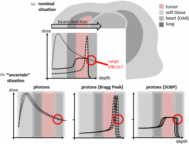
Figure 1. (a) Potential dose benefit of a proton treatment compared to a photon treatment (dotted line: photon depth dose curve; dashed line: mono-energetic proton depth dose curve known as Bragg Peak; straight line: spread out proton Bragg curve (SOBP) to cover the whole tumour). (b) Influence of uncertainties to these depth dose curves.
Download figure:
Standard image High-resolution imageIt is well recognized that this well-defined range is the main advantage of protons for radiotherapy. However, due to the steep dose gradient at the distal edge of the Bragg peak, uncertainties in determination of this range can have a profound impact on the actually applied dose distribution. Indeed, this uncertainty is probably the main factor limiting the ability of proton therapy to spare healthy tissues to their maximum potential. For example, in standard proton treatments of prostate cancer, parallel-opposed lateral beams are almost exclusively employed, as such a beam arrangement is thought to be least affected by range uncertainties. However, such a lateral approach is also associated with the largest radiologic path lengths to the target, increasing the volume of irradiated normal tissues and also leading to increased lateral scatter and a consequently wider dose penumbra which generally will be higher than that which can be achieved using conformal photon treatments. An improved knowledge of proton range in vivo however, could result in increased confidence in the use of more 'adventurous' field directions that use the steeper distal fall-off to shield critical structures (like the rectum) and which would also have shorter path lengths through normal tissues. This improved dose conformity to the target and reduced normal tissue involvement, in turn, could allow for more dose escalation, whilst maintaining adequate sparing of healthy organs (Trofimov et al 2007). This simple example emphasizes that it would be extremely desirable to measure proton ranges directly in vivo.
Spurred on by this desire, over the last years, many different approaches for in vivo proton range verification have been proposed and investigated and it is the aim of this article to review these.
Throughout this review, we will categorize the different approaches in the following ways:
Measurement technique
Direct: methods by which range is directly measured
Indirect: methods by which proton range is implied from another signal
Timing
Online: methods which can be performed during, or immediately before treatment delivery
Offline: methods that can only be performed after completion of the treatment
Dimension
1D: single (or few) point measurements
2D: two dimensional (imaging) measurements
3D: three dimensional (volumetric) measurements
The review is organized as follows. In section 2, the basic physics of proton interactions with tissues will be reviewed, and a brief description given of the main modes of treatment delivery and associated treatment planning issues. In this section, we will also outline the main sources of range uncertainties that can affect the accurate prediction of proton range in vivo. Section 3 then reviews and discusses the different in vivo range verification methods that have been proposed, whilst in section 4, the current status from the point of clinical implementation, together with the potential and further directions of the different approaches are summarized and discussed. We conclude with an outlook and some final remarks in section 5.
2. Proton therapy physics, delivery and sources of range uncertainty
2.1. Proton interactions with matter
2.1.1. Energy loss
Protons passing through matter mainly interact with electrons via electromagnetic Coulomb interactions, by means of which they continuously lose energy. The rate of loss of energy increases with increasing depth of penetration. The energy loss due to Coulomb interactions in a medium with a density ρ is described through the stopping power S(E) of charged particles with energy E:
For charged particles with masses much larger than the electron mass me, S(E) is analytically described by the Bethe–Bloch equation (Bethe 1930, Bloch 1933). For protons it reads
The kinematic terms β and γ are defined as  and
and  ; Tmax denotes the maximum transferable energy to an electron and I is the mean ionization potential of the particular medium with the nuclear number A and the atomic number Z. The decrease of energy loss for charged particles in material as a function of the increasing velocity v becomes apparent through the approximate relation
  . The Bethe–Bloch equation together with the statistical nature of the Coulomb interaction for an ensemble of protons (Oelfke et al 2002) leads to their characteristic depth dose curve with a low entrance plateau and a steep distal peak, known as the Bragg curve (Bragg and Leeman 1904) (see figure 1(a)).
2.1.2. Multiple Coulomb scattering
In addition to energy loss, protons are laterally scattered through three processes. The first (and least important) is the deflection through Coulomb interactions with electrons. However, as protons are 1800 times heavier than electrons, this is a small enough effect that it can be effectively ignored. Much more significant are the effects of Coulomb interactions with atomic nuclei, an effect known as multiple Coulomb scattering (MCS). In this process, when protons pass close enough to the nuclei, they are deflected (repulsed) through the electrostatic forces resulting from the positive charge of the proton and the likewise positive charge of the nucleus. Finally, primary protons can also be deflected through in-elastic collision directly with the nucleus (see below). As a rule of thumb, the contribution to the width of the beam at the Bragg peak due to MCS alone is approximately 2% of the range of the Bragg peak in water (Goitein 2008).
2.1.3. Nuclear interactions
In addition to energy loss through interactions with electrons, and track deflections through Coulomb interactions with nuclei, there is a small, but finite probability that the primary protons will interact directly with atomic nuclei through elastic and inelastic nuclear interactions. In elastic collisions, the nuclei are left intact, and the primary proton will be deflected, whilst in in-elastic collisions, the protons will be lost from the beam, and the characteristics of the nuclei changed. Due to such interactions, 1% of protons are lost per cm of range in water. However, more importantly, a consequence of such in-elastic nuclear interactions, is that short-lived radio-isotopes are created (e.g. for proton irradiations predominantly O15 and C11, both positron emitters). As we shall see below, the production of such isotopes by proton irradiation can be directly used to infer particle range in vivo.
2.2. Delivery modes
The advantageous characteristics of protons have been clinically used since the 1950s and, at the time of writing, have been applied to nearly one-hundred thousand patients worldwide (see PTCOG website). Protons can be delivered for radiotherapy using two main modes. The most mature method, and currently still the most widespread, is known as passive scattering (Koehler et al 1977, Grusell et al 1994). In this approach, scatter foils are used to broaden the narrow proton beam extracted from the accelerator into a broad beam suitable for therapy. This broadened proton field is then shaped to the geometry of the target by the use of an aperture (for lateral dose conformation), a range compensator (for distal conformation) and a range modulation device for spreading the dose along the beam direction to form a so-called spread-out-Bragg-peak (SOBP) (see figure 1(a)). The second approach is known as active scanning. Here a narrow and quasi-mono-energetic proton 'pencil' beam is magnetically scanned across the target, in combination with step-wise changes of the energy to scan the Bragg peaks also in depth. Indeed, scanning exists in many flavours, from discrete spot scanning (Kanai et al 1980, Pedroni et al 1995), through raster scanning (Kraft 2000) to continuous line scanning (Zenklusen et al 2010).
In general, scanned proton fields have the advantage of greater target dose conformity, require less (or even no) patient-specific hardware and significantly reduce the neutron contamination compared to passively scattered proton fields (Schneider et al 2008). Furthermore, scanning offers the possibility of delivering intensity modulated proton therapy (IMPT) (Lomax 1999 and 2008), which can further increase the conformity of treatments as will be explained briefly in the following section. On the other hand, it is technically difficult to produce (and transport through a beam-line/gantry system) very narrow pencil beams such as to maximize lateral dose fall-off and in addition, scanning is also extremely sensitive to organ motion (Phillips et al 1992, Bortfeld et al 2002).
2.3. Treatment planning
Treatment planning in proton radiotherapy mostly employs analytical pencil beam models. Pencil beam algorithms rely on facility-specific pencil beam kernels to accurately model proton range mixing from range straggling and beam broadening due to MCS along the whole beam path (Goitein and Miller 1983). The calculated proximal build-up, distal fall-off and lateral penumbra are usually in good agreement with measurements, at least in water (Hong et al 1996), although, as with all analytical calculations, there are limitations to the accuracy of these approaches when being delivered in patients, due to the complex density heterogeneities involved (Urie et al 1986). In addition to pencil-beam based algorithms, Monte Carlo dose calculation procedures have also been developed, although these are mainly used in research (Paganetti 2006, Paganetti et al 2008, 2012). They are believed to be more accurate (Pawlicki and Ma 2001) but usually take too much computing time to be used in routine treatment planning.
As with photons, proton treatments use multiple portals to reduce the overall skin dose to patients and also to reduce the sensitivity of the plans to range uncertainties (see above). However, as individual proton fields can be so designed such as to deliver a more or less homogenous dose to the target from a single field direction, treatment strategies and treatment options can be somewhat different from those of conventional therapy. For instance, if each treatment field contributes a uniform dose within the target, the corresponding treatment plans are typically named single field, uniform dose (SFUD) plans. In contrast, IMPT is a treatment technique that, in analogy with intensity-modulated radiotherapy (IMRT), delivers intentionally non-uniform dose distributions from each treatment field. The desired (generally uniform) dose in the target volume is then obtained after superimposing the dose contributions from all fields. The additional degrees of freedom (by not having to produce uniform dose from each direction) can be used to optimize dose distributions in several ways and with usually improved sparing of neighbouring critical structures (Lomax 2008).
However, it should also be noted that a type of IMPT can also be achieved in passive scattering, and indeed has been used for many years clinically. This approach is called 'field patching' (Bussiere and Adams 2003). In this approach, two or more passively scattered fields are combined such that the first field treats a segment of the target whilst avoiding a nearby critical organ with its lateral penumbra. Subsequent fields then treat the remaining, mainly un-irradiated segment, such as to also avoid the critical structures, but with a matching of their distal dose fall-off to the lateral fall-off of the first field as seen in figure 2(c).

Figure 2. Different planning strategies for proton therapy and their potential sensitivity towards range uncertainties.
Download figure:
Standard image High-resolution image
2.4. Consequences and sources of range uncertainty
For all treatment techniques in proton therapy, the reliability on an accurately determined penetration depth is essential, and much more so than for photons (Schlegel et al 2005) (see figure 1(b)). For instance, because often the sharpest dose fall-off of a proton field is the distal fall-off, it is theoretically possible, and extremely tempting from results of treatment planning alone, to aim proton fields directly against critical structures. However, due to uncertainties in the exact proton range (see below), this is rarely done in practice, due to fears about significantly overdosing the distal structure as a consequence of potential overshoot of the distal gradient into the structure.
This is demonstrated in a schematic way in figure 1(b). This compares the expected changes in the delivered doses of a photon (left) and proton (right) field in the case that a density heterogeneity in the beam path would be ignored in the treatment planning process. In the case of photons, this results in a reduced dose beyond the heterogeneity of only a few percent. However, for the proton SOBP field, the same 'error' in calculation could result in changes of doses of up to 100% due to the extremely sharp dose gradient in the distal edge of the SOBP. Although such an example is extreme (all modern proton therapy planning is based on CT data sets and so such a simple geometry should be modelled quite accurately), as we shall see below, there are a number of reasons why an exact calculation of the range in the patient is extremely difficult. However, even if 'ranging out' on critical structures is avoided, IMPT and patched passively scattered treatments are nevertheless still sensitive to range uncertainties, due to the potentially sharp distal gradients of the individual fields that are expected to 'patch' to lateral fall-offs of other fields as seen in figure 2 (Lomax 2008, Albertini et al 2010).
So, uncertainties in proton range can have a profound effect on proton treatments. But what are the sources and reasons for range uncertainties in vivo?
As in conventional radiotherapy, computer tomography (CT) data sets are the basis of treatment planning and range calculations. As such, range calculations are limited by the inherent limitations of CT image acquisitions. For instance, image noise (less so) and beam hardening issues (more so) will directly affect range calculations. These will be compounded by partial volume effects and also reconstruction artefacts, the latter of which can be huge in the presence of metal implants such as tooth fillings or surgical implants (Newhauser et al 2007, Jaekel and Reiss 2007). In addition, CT Hounsfield values (HU), giving as they do the relative attenuation of x-rays of the tissue in relation to water, must first be converted to relative proton stopping powers before proton ranges can be calculated. Although sophisticated algorithms have been developed for the generation of such calibration curves (Schneider et al 1996, 2000), there are inevitable uncertainties associated with these curves, not least the problem that the actual conversion is dependent on the chemical composition of the material, and not just on its HU value. Thus, two materials with the same HUs can have quite different proton stopping powers and vice versa. When based on good quality CT images, errors due to this conversion alone have been estimated at ±1.1% for soft tissues and 1.8% in bone (Schaffner 1997), and in total, it is generally assumed that range uncertainties based on a good quality, well calibrated CT are of the order of ±3% (Moyers et al 2001). In addition, there is an inevitable uncertainty in the relative biological effectiveness (RBE) of low-energy protons, which correspond to an uncertainty in biological range of a few mm (Paganetti 2003, Carabe et al 2012), however this will not be considered further in this review.
In summary, all the above uncertainties are almost certainly systematic in nature, as a treatment plan is generally based on a single CT acquisition and a single calibration curve. Thus, uncertainties in ranges from the CT alone will likely be the same for every delivered fraction of a treatment.
Moving on, there are two more sources of range uncertainty which, however, can be considered to be random in nature. The first are variations in the delivered proton energy on a day-to-day basis and the second, range changes due to variations in patient positioning in relation to the beam. The magnitude of the first is generally very small (typically much less than 1%), whilst the uncertainties in range from positioning errors can be quite substantial, particularly when treating through areas of large density heterogeneities and/or patient surfaces that are oblique to the beam direction. However, both of these uncertainties can be considered to be random in nature, i.e. they will change on a day-to-day basis, and thus will tend to 'blur' out under normal fractionation conditions, unless, of course, radio-surgery or hypo-fractionated treatment regimes are being used.
This is not the end of the story however. If conventional fractionation schemes are adopted, a typical course of proton radiotherapy will take place over many weeks. Although this may help in some circumstances (e.g. to reduce the effects of daily positioning errors, see above), it has other, potentially major disadvantages. Over such a timescale, patient anatomy can change significantly, whether this is due to tumour mass reduction, weight loss/gain (see e.g. Albertini et al 2008) or daily changes in the filling of internal cavities (nasal cavities, bowel/rectum/bladder filling, etc). Although some of these could be considered to be random in nature, the magnitudes of these effects can be substantial, and for some (e.g. weight loss/gain, tumour shrinkage), these can change slowly and systematically through the whole treatment course.
In short, there are a number of reasons why proton range in the patient is uncertain and strongly emphasizes the need for accurate methods of verifying range in vivo.
2.5. Current approaches to managing range uncertainty in proton therapy
The goal of treatment planning is to find the optimal dose distribution in terms of dose conformity, healthy tissue sparing and robustness towards any uncertainties. In conventional radiotherapy with high-energy x-rays, 'robust' planning (robust for the tumour volume at least) is generally achieved through the use of margins. In proton therapy however, the concept of the planning target volume (PTV) is somewhat more complicated. This is due to, amongst other things, the breakdown of one of the underlying assumptions behind the PTV concept, i.e. that the form of the dose distribution itself does not change substantially due to positioning errors, but simply shifts in relation to the target volume. This is not necessarily true for proton therapy, as patient positioning errors can also result in changes in the proton range for the case where local density heterogeneities move in and out of the beam due to these errors. In addition, as described above, there are inevitable range errors from the planning/dose calculation process itself which are present even for a perfectly positioned patient, and these are very likely systematic in nature. The potential consequences of this from the point of view of PTV margins can be seen by referring to the van Herk formula for margin determination (van Herk et al 2000). The margin calculation has two components, originating from the magnitude of the estimated random and systematic errors of the treatment, which are very differently weighted. Whilst the magnitude of the random error is weighted by the factor of 0.7 in the formula, systematic errors should be weighted by the factor of 2.5. Thus, in principle, we should have substantially larger margins at the distal end of the target volume to deal with range errors (being mainly systematic) than are required laterally, which are mainly determined by patient positioning issues and are therefore mainly random in nature. This inevitably leads to the need for 'field specific' PTVs (Rietzel et al 2006, Thomas 2006), and margins with potentially large magnitudes in the distal direction. Although at the time of writing, we are not aware of any centre which is routinely working with field-specific PTV margins, and certainly not calculated using the van Herk formula, this example indicates the high degree of complexity potentially involved in margin calculations for proton therapy.
In proton therapy, the potential effects of range uncertainties are also managed by other means. One way is the careful selection of field arrangements (Lomax et al 2001). For example, the influence of range uncertainties on critical structures can be minimized by sparing them using lateral field edges rather than distal, and (for passive scattering) by field patching, where distal and lateral fall-offs can be matched to form concave dose distributions around critical structures. For such field combinations, the use of different junctions and field combinations on different days ensures that potential dose in-homogeneities due to misalignment of these edges can be reduced over the whole treatment. In addition, Moyers et al (2001) have proposed to abandon the PTV concept and suggested that corrections should be made by adjusting the beam-specific hardware, such as the compensator and aperture, which effectively then becomes a field-specific alternative to the PTV. For instance, uncertainties caused by tissue density misalignments (Urie et al 1986) could be compensated by modification of the compensator using 'smearing' techniques. In addition, Albertini et al (2011) have also questioned the usefulness of PTV margins for IMPT treatments, and other authors have proposed that the best method of dealing with uncertainties in proton therapy is through the use of 'robust' optimization methods (see e.g. Unkelbach et al 2007, 2009, Albertini et al 2010). Whatever approach is used however, there will always be a desire to monitor and verify the success of these methods in the patient with in vivo proton range verification.
3. Methods for verifying range in vivo
Given the perceived importance of in vivo range verification, it is perhaps not surprising that a number of different approaches have been proposed in the literature. In order to organize our review of this area, we divide these methods into direct and indirect approaches, as defined in section 1 above. In short, direct methods directly measure proton range by direct dose or fluence measurements, whereas indirect approaches imply particle range from surrogate signals resulting from the proton irradiation.
3.1. Direct methods
3.1.1. In vivo point measurements
Timing: On-line
Dimension: 1D
In vivo point dose measurements have been widely used for verifications in photon/electron treatments (Essers and Mijnheer 1999). Recently, an implantable dosimeter with a wireless readout became available and has been investigated for photon-based treatments of prostate cancer (Black et al 2005, Beyer et al 2007, Scarantino et al 2008). This has initiated the investigation of the use of similar detectors for in vivo range verification in proton therapy.
For passively scattered proton fields, a (integrated) point dose measurement does not provide much information about the particle range. At any position within the target volume, a point dose measurement will always result in the same value, as a homogenous dose is usually delivered to the target. On the other hand, due to the steep dose fall off at the end of the proton depth dose curve, a measurement at the distal edge of the target will be very sensitive to the positioning of the detector, which is difficult to determine exactly in vivo. To overcome these challenges, two approaches have recently been proposed.
Lu (2008a) has proposed the use of in vivo, point based, time dependent dose rate measurements. It was shown that the time dependence of a delivered SOBP is unique at every point in depth and thus encodes the depth information. If the time dependence can be acquired at a point in the patient, a 'decoding' can be performed to obtain the residual range of the beam at this position. While originally proposed for passively scattered proton fields, the method can also be adapted for actively scanned proton treatment fields, since here also, with each position in the target, a specific time-delivery characteristic is associated. This approach was first tested using a small ionization chamber (IC) (Lu 2008a), whereas in a more recent publication, semiconductor diodes have been proposed as an alternative (Gottschalk et al 2011). They have the advantage of being two-terminal devices which do not require a bias voltage and which are small, rugged and inexpensive. For an eventual clinical implementation, an array of diodes spread over a few cm2, perhaps on a flexible membrane attached to a rectal balloon, is envisioned. For both detector types, it was shown that the root mean square (rms) width σt of the dose burst, associated with a single modulator cycle, provides sub-millimetre precision for determination of the proton range at a specific position. These tests, however, were performed in the ideal environment of a single, precisely oriented diode in a homogeneous water phantom. Using blocks of materials equivalent to bone, air and water the robustness of the method was tested against range shifting and range mixing (Bentefour et al 2012). For pure range shifting, its accuracy was found to be better than ±0.5 mm and reasonable results were also found for range mixing. In a patient however, the ultimate precision and accuracy of the method will be dominated by more complex heterogeneity effects and the exact determination of the detector position. Thus, this approach remains to be proven to be practical and precise in real clinical situations.
For the second method, also proposed by Lu (2008b), the authors suggest to replace the conventional SOBP field by a complementary field pair, each with a deliberately sloped depth dose profile. In this case, the ratio between the two distributions can be a sensitive indicator of radiological path length. Measuring this ratio at a point inside the target volume can thus provide the water equivalent path length at the dosimeter location. This second method requires only a dose measurement without any additional time information and may therefore be simpler to implement clinically. Although this approach was only discussed for passively scattered proton fields, a sloped dose characteristic just as easily can be produced by actively scanned proton beams. In fact, the ratios between the individual pencil beam layers could be utilized in a similar manner with even more flexibility (Lu 2009) and given the complexity of the individual field dose distributions for IMPT plans, this method could be very interesting for this treatment modality.
Using the only commercially available implantable dosimeter with wireless reading (dosimetry verification system (DVS) Sicel Technologies Inc., Morrisville, NC) this method has also recently been tested experimentally (Lu et al 2010). DVS dosimeters are metal oxide semiconductor field effect transistor (MOSFET)-based radiation detectors and are known to have a dependence on linear energy transfer (LET) (Rosenfeld et al 2000). Due to this LET dependence, DVS detectors do not measure a constant dose in the plateau area of a conventionally delivered SOBP field. Indeed, this dependence could also be used for range verification. However, the DVS–dose curve becomes steep only near the distal end of the SOBP, requiring precise positioning of the dosimeters. This is, as mentioned previously, difficult to achieve in clinical practice. Using the LET dependence for range estimation would also require an absolute calibration of the MOSFET detectors. Lu et al (2010) developed a method based on the columnar recombination model to correct for LET dependence. For sloped proton treatment fields, it was shown that the DVS dosimeters can measure dose ratios with a relative uncertainty of 1–3% at various depths.
The use of implantable dosimeters makes range verification during the delivery of each field possible. It requires no additional time for the patient and gives the same dose distribution as planned. However, the forms of the individually delivered fields have to be modulated in order to allow for the range measurement. An obvious limitation of any approach based on point measurement is the fact that it can only verify the range at a limited number of points (Lu 2008a). Clearly, this would not be sufficient for treatment sites that require range verifications at finer resolution, due to, for example, tissue inhomogeneities along the beam path and/or inside the target volume. Severe tissue inhomogeneities can also distort the dose distribution through multiple scattering and degradation of the distal edge dose fall-off. As a result, the depth–dose 'slope' in the patient, and thus the dose ratio function, may differ substantially from water tank measurements. In fact, the dose ratio may depend not only on the radiological depth, but also on the geometric position of the dosimeter, and therefore can no longer uniquely verify the beam range. Another limitation is the fact that the dosimeters must be inserted inside the target volume. Hence they only verify the beam path from the body surface to the locations of the dosimeter, rather than to the distal surface of the target volume. Nevertheless, the remaining part of the beam path is much shorter and its uncertainty should thus be much smaller, particularly for soft tissue targets. In addition, the implantation of markers may not be possible for many tumour types, thus limiting the applicability of this approach.
In summary, only tests in phantoms have been carried out using in vivo point measurements, and the submillimetre precision found in these tests has yet to be confirmed in clinical studies in patients.
3.1.2. The range probe
Timing: On-line
Dimension: 1D
In vivo implanted markers provide a 1D range signal measured at a limited number of points within the patient. As mentioned however, it relies on the possibility of implanting the dosimeter directly in the patient, ideally close or within the tumour, which is not always possible and is invasive for the patient. An alternative 1D range measurement is the concept of the 'range probe' (Romero et al 1994, Watts et al 2009, Seco and Depauw 2010, Mumot et al 2010). In this case, a single proton pencil beam of sufficient energy to pass completely through the patient is applied, and its residual range then measured on its exit from the patient. This has two main advantages. First, by using a multiple layer ionization chamber (MLIC) (Yajima et al 2009), the complete Bragg peak can be measured, including potentially a high-resolution (in depth) measurement of the distal gradient. As shown in the work of Mumot et al (2010), this could lead to in vivo range estimates at the 0.5% level, based on Monte Carlo simulations of range probes through example CT data sets. In addition, only plateau dose is delivered in the patient, meaning that the doses delivered from such range probes can be very low. Subsequently, it is foreseeable that multiple range probes could be applied from any direction, and the authors make the suggestion that, through careful selection of the range probe positions, it could then be possible to both validate in vivo range and to estimate patient positioning errors by measuring the changes in Bragg peak shape in relation to density heterogeneities as a function of positioning offset. Ultimately, it would also be feasible to deliver many hundreds of such range probes, each separated by a few millimetres to perform a low-resolution proton radiograph (see next section) (Telsemeyer et al 2012).
The main advantage of this approach is that it is relatively simple, and requires only a MLIC as a detector, which is available commercially. The main disadvantages are the requirement for higher energy protons (maybe higher than 250 MeV if measurements need to be made laterally through the pelvis), poor spatial resolution and the fact that only the total range change through the whole patient can be measured, and not the range directly at the tumour position. On the other hand, for the same reason, range uncertainties derived from such a technique can be considered to be 'worst case' estimates and can potentially give valuable information about the accuracy of the CT/calibration curve data.
3.1.3. Proton radiography and tomography
Timing: On-line
Dimension: 2D/3D
Proton radiography has been investigated since the late 1960s, and is the 2D extension of the range probe concept. That is, higher energy protons are applied to the patient, which are then detected on exit from the patient, from which the residual range can be directly measured. However, in radiography, a 2D fluence of protons is used and, in order to obtain improved spatial resolution, the entrance and exit coordinate of each proton is detected in coincidence with the range measurement (Schneider and Pedroni 1995). Thus, the set-up for high-resolution proton radiography is somewhat more complex than for the range probe described above.
Historically, proton radiography first caught attention because of its high contrast (Koehler 1968, Steward et al 1973a, 1973b). Early on, it was reported that high-contrast images obtained by proton radiography provided improved imaging of low-contrast lesions over conventional x-ray techniques (Kramer et al 1977). Furthermore, comparisons of proton radiographs with x-ray radiographs showed that the use of protons has a dosimetric advantage (Moffett et al 1975) and in the mid-90s, a reduction of imaging dose by a factor of 10 to 20 was reported for protons as compared to x-rays (Schneider and Pedroni 1995). The newest publications state that for radiographs of equal spatial and density resolution, 50–100 times lower image exposure for protons can be achieved (Schneider et al 2004). In the context of this review, the most interesting justification for the use of proton radiography is given by the fact that it directly provides stopping power values of the tissue, which are the basis for treatment planning in proton therapy (Penfold et al 2009). When conventional x-ray images are used, the measured electron densities have to be converted into stopping powers which introduces uncertainties (section 2.4). Thus, proton radiography offers an in vivo range measurement that can be used for treatment planning and/or range verification during the course of treatment.
Despite these advantages, proton radiography has not progressed rapidly, mainly due to source availability and cost (Cookson 1974, Kramer et al 1977). To obtain optimal imaging quality, the proton beam has to have specific characteristics, which will be discussed in detail later on. On the other hand, proton beams are easier to understand quantitatively and allow the use of inexpensive detector systems with 100% quantum efficiency (Kramer et al 1977). Since nuclear interactions occur rarely, dosimetric measurements of protons are easier and more accurate than those of x-rays.
The main disadvantage of proton radiography is the limitation in spatial resolution due to MCS, a limitation already identified in the first publications (Koehler 1968, Moffett et al 1975). Protons undergo numerous small angle deflections caused by their interactions with the Coulomb field of the nuclei in the traversed material, which produces uncertainties in the reconstructed proton trajectory (Schneider and Pedroni 1995, Schneider et al 2004, 2012, Penfold et al 2009). The achievement of a spatial resolution up to 1 mm has, however, been reported. Schneider et al investigated the impact of various proton measurement arrangements on the spatial resolution. In particular, they considered different combinations of entrance and exit coordinates, angle measurements, initial particle energy and angular confusion of the incident proton field. It was found that the best resolution is obtained by measuring, in addition to entrance and exit coordinates, also entrance and exit angles, and in general, that one can improve the spatial resolution by increasing the proton energy.
Three distinct physical phenomena can be used to measure residual range or energy (Cookson 1974). In 'marginal range radiography', the rapid fall in proton intensity near the mean range is employed. In the 'density profile and porosity measurements', the energy lost by individual protons is used, whereas in 'multiple scattering radiography', the angular spread given to a proton beam as it traverses the material gives the desired information. Most interesting in the context of this review paper are the first two approaches, which have also appeared most often in the literature. When comparing the transmission curves of protons and x-rays, it is obvious that by using the steep portion at the end of the proton curve, changes in transmission need to be measured less accurately than for x-rays to detect a given change in thickness or mass (Kramer et al 1977). A detector which is placed near the end of range of a monoenergetic proton beam is therefore very sensitive to changes in the mass of material that is traversed and the detector will see large intensity changes for small mass changes in the sample (Moffett et al 1975). In order to detect larger mass changes in this approach, a stack of detectors has to be used (about range probe above) leading to rather bulky systems. More compact detectors however, can be used if the density information of a sample is derived from the residual energy of the traversing protons. In this case the density resolution is directly related to the energy resolution of the detector. In addition, proton radiographs contain quantitative information on the range and the range dilution. Range dilution images can be helpful in estimating safety margins around the target volume and to find optimal beam directions for radiotherapy.
Optimal proton beam characteristics for radiography have first been pointed out by Moffett et al (1975). Ideally a small pencil beam should be used with an intensity of about 108 s−1. The beam should have an energy spread of less than 1/4%, and a short-term stability of 1/200%. At least 100 protons per pixel are needed to achieve good density resolution. In practice, density resolutions of 0.5 mm have been demonstrated in animal measurements (Schneider et al 2004) and proton radiographs of about 20 cm × 20 cm can be acquired in approximately 20s depending on the beam delivery parameters and the detector efficiency.
As with the range probe, proton radiographs detect range variations for the whole body diameter, whereas one is more interested in the range variation caused by protons stopping at a specific location in the body in a treatment situation. Nevertheless, radiographic measurements can give an upper limit on the range error which can occur during treatment (Schneider and Pedroni 1995). Proton transmission imaging can also be extended into 3D tomography mode. Consequently, range verification is theoretically possible in 3D as well, although the main interest in proton tomography at the moment is for treatment planning purposes to more accurately (and directly) measure stopping power for range and dose calculations (Cormack and Koehler 1976, Schulte et al 2002).
Proton transmission measurements are the most direct way of obtaining range verification information. Since proton transmission images can be taken under the same geometrical conditions as the treatment, the images are true proton-beam's-eye-view projections (Schneider and Pedroni 1995). In addition, due to the low dose, imaging can be done for each fraction and could be used to detect changes of the anatomy during treatment, for example decreases of target volume or changes in patient weight. Besides its potential for range verification, proton transmission imaging has also been proposed for patient set-up verification (Romero et al 1994, Schneider and Pedroni 1995).
Despite the substantial capability of proton transmission imaging to serve as a range verification tool, it is currently not being used clinically, and is not being provided by any particle therapy manufacturer (Mumot et al 2010). However, proton radiographs of an animal patient have been obtained under clinical conditions and in a clinically acceptable time with satisfying spatial and density resolution (Schneider et al 2004). Interestingly, there is one facility worldwide that performs high-energy proton therapy (Abrosimov et al 2006) for which 2D proton radiographs could be performed. Nevertheless, no research intention or results on this topic have been reported by this group. Although research proposals for 3D proton tomographs have been published (Schulte et al 2002), clinical implementation is still a distant prospect. Nevertheless, given the rapidly increasing number of proton therapy centres worldwide, further investigations are without doubt worthwhile.
3.2. Indirect methods
3.2.1. Prompt gamma imaging
Timing: On-line
Dimension: 2D/(3D)
While passing through tissue, protons undergo nuclear reactions, some of which result in the emission of gammas. There are two kinds of gammas that can be used for treatment monitoring (Min et al 2006): (1) coincident gammas from the production of positron emission isotopes and (2) prompt gammas from excitations of the target nuclei. The former method makes use of conventional positron emission tomography (PET) and will be discussed below. The second method, prompt gamma imaging, was actually mentioned first in the context of the PET imaging approach (Parodi et al 2005) where prompt gamma-rays represent noisy events that are difficult to separate from the decays of long-lived beta+-emitters, which generate the signal used in the PET approach. However, the direct employment of prompt gammas for range verification was first proposed by Min et al (2006).
Inelastic interactions of protons and target nuclei occur along almost the whole proton penetration path, until 2–3 mm before the Bragg-peak, where the reaction cross sections start dropping with decreasing energy of the projectiles. After an interaction, the target nucleus is excited to a higher energy state and then emits a single photon (prompt gammas) to return to its ground state. Thus, the emission of prompt gammas is correlated with the penetration path of the protons in the tissue, so that measurements of the prompt gammas can be used to draw conclusions on the proton range. However, it is important to realize that the prompt gamma falloff is not equal to the dose falloff. Only a consistent and predictable fall-off difference enables proton range verification (Moteabbed et al 2011). The emission spectrum of the prompt gammas is in the range of MeV (2–15 MeV) and is dominated by a number of discrete gamma-lines from specific nuclear de-excitations. When looking at the energy spectrum, more low, rather than high, energy gammas are produced and discrimination of the distal dose falloff is easier for high-energy gammas (Min et al 2006, Kurosawa et al 2012). This is for two main reasons. First, higher energy gammas experience less scattering effects on their way out of the target and second, the production of higher energy gammas has improved localization in relation to the dose falloff.
The main advantage of prompt gamma imaging is the ability to perform real-time verification of proton dose delivery. The isotropic prompt gammas can be detected instantaneously, within a few nanoseconds, following the nuclear interactions. Even the application of a therapeutic dose of 2 Gy min−1 results in a sufficiently high production rate of gammas. Furthermore, prompt gamma imaging enables treatment monitoring without additional dose.
In their first publication, (Min et al 2006) reported the position verification of the Bragg peak of a 100 MeV proton beam in a phantom with an accuracy of 1–2 mm. During the last years, various groups have been able to confirm this result, and have also performed measurements and Monte Carlo simulations using custom-built prototype detector systems. In particular, different groups have demonstrated the feasibility of the approach for monoenergetic proton pencil beams over the whole domain of clinically relevant proton energies (Polf et al 2009a, Kabuki et al 2009, Styczynski et al 2009, Peterson et al 2010, Frandes et al 2010, Kurosawa et al 2012). Thus, the practicability of in vivo prompt gamma range verification for scanned proton beam therapy has been demonstrated. There has been doubt, however, if verification of each individual pencil beam of a treatment field is feasible. Lower proton numbers at low-weighted spot positions (occurring for optimized proton fields or IMPT) could result in an insufficient prompt gamma signal. Lower spot weights, however, usually occur at proximal spot positions in the field, where the reduced gamma production due to a reduced proton number is possibly compensated by the increased gamma production rate of low-energy protons (Polf et al 2009a).
Theoretically, the feasibility of range verification for passively scattered SOBP fields has also been demonstrated (Polf et al 2009a, Moteabbed et al 2011). However, in measurements performed with a collimated detector system, the gamma falloff at the position of the dose falloff disappeared (Kurosawa et al 2012). This is probably due to background neutrons and stray gammas that blur the location of the distal dose falloff. Future studies have to show if other detector systems might be able to cope with these challenges.
The clinical application of prompt gamma range verification has failed so far mainly due to the absence of an optimized prompt gamma detector. Conventional single photon emission computed tomography (SPECT) is not feasible because of the high energy of the prompt gamma emission spectrum which would require impractically thick collimators. Hence, various alternative approaches are being pursued. Several dedicated research groups have reported promising results on prompt gamma detector developments within the last few years.
The most straightforward approach that has been investigated is the collimated prompt gamma camera (Min et al 2006, Testa et al 2010, Kurosawa et al 2012, Bom et al 2011). As mentioned above, in early setups this approach was challenged by neutron background radiation and stray gammas, necessitating thick layers of collimation. MC simulations imply however that array-type setups would allow for the measurement of prompt gamma distributions from therapeutic proton beams (Min et al 2012). On the other hand, a recent publication by Bom et al (2011) claims that challenges could be solved by using a gamma camera in combination with a knife-edge shaped slit placed perpendicularly to the beam direction. In MC simulations they show that under common therapy conditions for proton spot scanning, enough data during one spot can be collected to enable location of the distal dose edge with a 1 sigma accuracy of better than 1 mm. A first prototype slit camera was prepared and tested successfully at 100 and 160 MeV proton beam energies by Smeets et al (2012). Another solution to overcome the challenges of detection could be the additional employment of time of flight (TOF) techniques to differentiate the prompt gamma component from the background radiation. The TOF method would make bulky shielding around the detectors unnecessary. This means a series of thin detectors, each of them aligned to a corresponding collimator slit, could be stacked. Such a setup allows as many detectors as needed to cover the entire longitudinal range of protons (Testa et al 2010). In order to perform 2D dose cartography with this setup, a position sensitive hodoscope can be used.
Compton cameras however seem to be emerging to be more suitable for in vivo prompt gamma range verification (Kormoll et al 2011). Their main advantage over collimated gamma-cameras is an increased efficiency of potentially up to two orders of magnitude. This is due to the replacement of the performance-limiting absorbing collimators by an electronically operating collimator. In the literature, mainly double scattering Compton cameras have been studied (Seo et al 2007, Peterson et al 2010, Kormoll et al 2011, Richard et al 2011). They enable direct analytical reconstruction, which is otherwise not possible because high-energy gammas do not deposit all their energy in the camera detectors. Furthermore, double scattering Compton cameras show an improved spatial resolution. Compton cameras have also been used with a beam hodoscope for particle tagging (Richard et al 2011). The beam tagging device has a dual function: first, it gives a time reference for TOF measurements performed in order to discriminate the gamma signal from the background. Second, it makes it possible to tag the incident ions spatially in the plane transverse to the beam. Therefore, the reconstruction of the prompt gamma image is expected to be simpler.
Guidelines for the design of a double scattering Compton camera have been discussed in the literature (Peterson et al 2010, Richard et al 2011). Setup parameters like detector spacing and detector thickness were investigated in order to optimize the detection efficiency for prompt gamma rays in the energy range of 2–15 MeV. For the scattering component, as well as for the absorber part of a Compton camera, different materials have been proposed. Compton cameras using gas chambers however might be the most promising approach in terms of clinical implementation. They are capable of tracing scattered electrons and therefore are named electron tracking Compton cameras (ETCC). ETCCs have the merit of projecting the incident gamma direction by a single scattering event and are capable of reliably rejecting background gammas and neutrons. Furthermore, they can image proton dose in 2D. Applicability investigations of ETCCs for medical imaging using a low-energy gamma source were reported by several groups (Takada et al 2005, Kabuki et al 2001). More recently, studies for gammas in the energy domain relevant for prompt gamma imaging studies have been performed (Frandes et al 2010, Kurosawa et al 2012). An alternative approach is to use 'gamma electron vertex imaging' (GEVI), in which the high-energy gammas from a source are first converted by Compton scattering to electrons, which subsequently are traced to determine the location of the gamma source. In simulations, proton beam ranges within 2–3 mm error could be verified in simple geometries (Kim et al 2012).
Besides using the prompt gamma signal for range verification, the possibility of using the emitted gamma spectrum to determine the elemental composition of irradiated tissue has also been investigated (Polf et al 2009b). This could provide a method for analyzing changes in the tissue composition in vivo during irradiation, or from treatment fraction to treatment fraction. For example, changes in the level of tumour hypoxia over the course of treatment could be monitored this way. Currently, however, this approach is also impaired by the unavailability of a suitable detector.
Recently instead of using prompt gammas, the use of proton-induced bremstrahlung radiation has been proposed (Yamaguchi et al 2012), which is thought to be more efficient due to its larger emission intensity. Monte Carlo simulations confirmed the feasibility of the method; however in practice, similar imaging devices as for the gamma approach would be needed, associated with similar challenges as described above. Experimental performance tests are planned in the near future (Yamaguchi et al 2012).
A comparison of prompt gamma imaging and PET imaging for in vivo proton range verification has been performed by Moteabbed et al (2011). Details of this study will be given below.
In summary, prompt gamma imaging for in vivo proton range verification has developed immensely from it first being proposed (Min et al 2006), with numerous groups working on the development of a clinically suitable detector system, and a number of detector systems already existing (Kabuki et al 2009, Frandes et al 2010, Peterson et al 2010). Since gamma imaging has a long history in several medical applications (PET, SPECT), as well as in many other areas of physics (astronomy, solid-state-physics), the wide know-how makes an early realization of an optimized detector system for prompt gamma imaging likely. Given a suitable detector system, this approach promises to enable very accurate, real-time range verification.
3.2.2. PET imaging
Timing: On-line/off-line
Dimension: 3D
As introduced in the previous section, and summarized in a recent review article (Studenski and Xiao 2010), range verification through in vivo PET imaging makes use of coincident gammas resulting from the annihilation of emitted positrons with electrons. When traversing tissue, a small fraction of protons create positron emitting isotopes (e.g. 11C, 13N and 15O) through nuclear interactions. The beta+-decay of these isotopes, or more precisely the recombination of the emitted positrons with an electron of the surrounding tissue, results in two coincident gammas that can be observed with a PET camera. The most relevant reaction channels and their characteristics, including the energy thresholds for the activation process, the isotope decay constant and the maximal kinetic energies of the emitted positrons are listed in table 1 in (Oelfke et al 1996). The corresponding half-lives of the isotopes are given in table 1 in del Guerra et al (1997).
The first suggestion of imaging-induced PET activity in radiotherapy was in connection with pion (Goodman et al 1986, Shirato et al 1989), neutron (Vynckier et al 1989) and heavy-ion therapy (Enghardt et al 1992). In the 90s, various groups (Litzenberg et al 1993, Vynckier et al 1993, Paans and Schippers 1993, Oelfke et al 1996, Litzenberg et al 1999) also started to investigate the use of PET techniques for in vivo dose monitoring of delivered proton doses. Clinically, this approach is appealing because it provides in vivo range information without additional dose cost for the patient.
For proton irradiation, beta+-activation solely results from induced target activation (no projectile activation). Therefore, the activation highly depends on the elemental composition of the underlying irradiated tissue (Parodi et al 2005a). In this manner, PET imaging with the goal of resolving the elemental composition of the irradiated tissue has also been investigated (Graffman and Jung 1975, Litzenberg et al 1999). The relation between the induced activity distribution and the dose distribution is not straightforward, due to its strong dependence on the elemental composition, i.e. the same dose distribution delivered to different inhomogeneous tissue geometries will result in different activity distributions. Therefore, attempts to verify the total delivered dose (Litzenberg et al 1999, Fourkal et al 2009) have so far failed. The relation between dose and activity is further complicated by the threshold energies for the production of beta+-isotopes that cause the activity distribution to drop prior to the dose distribution (Vynckier et al 1993, Oelfke et al 1996). Thus the fall-off positions of the activity and dose distribution are shifted against each other. Furthermore, the activity distribution changes depending on the timing of the PET imaging, due to the different half-lives of the active isotopes (Paans and Schippers 1993, Oelfke et al 1996). In perfused tissues, the activity signal also changes over time due to wash-out effects (Parodi et al 2007b, Knopf et al 2011). All these factors prevent a direct range verification by simply comparing dose and activity profiles and a comparison of measured activity distribution with a modelled activity distribution is required.
The spatial correlation of induced activity and dose was experimentally studied in polymer gel phantoms that exhibited a similar gross elemental composition to that of human tissue (Lopatiuk-Tierpak et al 2011). In homogenous (nonliving) tissue, knowing the elemental composition and the excitation cross-sections of the possible reactions, the expected activity distribution can be well modelled (Paans and Schippers 1993, Oelfke et al 1996). To precisely predict the measured distribution, the timeline of the data acquisition and the specific detector response have to be included in the model and cannot be achieved by simple stretching and weighting approaches (Parodi et al 2007) and therefore MC calculations have to be typically employed, and early reported activity measurements in phantoms (Litzenberg et al 1993, Oelfke et al 1996) have been validated against retrospective MC calculations by del Guerra et al (1997). Over the years, MC calculations have been advanced to also predict activity distributions in patients (living tissue) (Parodi and Enghardt 2000, Parodi et al 2002, Pshenichnov et al 2006, Espana and Paganetti 2010, Espana et al 2011). One limiting factor of MC calculations is the underlying cross-sectional data. It was reported that more experimental data is needed to reduce the uncertainties in MC simulations below 1 mm (Paganetti 2012). For patient simulations, a further crucial aspect is the knowledge of the elemental compositions of the different human tissues, which can be accomplished by a sophisticated conversion of Hounsfield units (HU) from the planning CT (Parodi et al 2007). Furthermore, CT-based Monte Carlo calculations have to be complemented by functional information, taking into account the metabolism of the induced positron emitters (Parodi et al 2007b). However, this is a complex process to model and only limited information from animal studies exists so far (Tomitami et al 2003, Mizuno et al 2003, Kitagawa et al 2006). Recently, the use of supplemental magnetic resonance imaging (MRI) data has been proposed to better resolve information about the local wash-out (Bauer et al 2011).
An alternative approach to MC simulations for predicting activity distributions is to convolve the planned dose distribution with filter functions, which can be derived analytically (Parodi et al 2006). In this approach, only the distal fall-off region of the PET signal can be predicted. This is, however, sufficient for the range verification of a proton beam. Furthermore, this approach can also be inverted, so that it permits the extraction of dose information from a measured PET distribution by the use of an inverse filter function. The filtering approach has been experimentally validated and further extended over the last years by Attanasi et al (2008, 2011). For the range verification in patients, both approaches are ultimately limited by the restricted knowledge about the elemental composition and the wash-out processes of different human tissues.
PET imaging of the induced activity can be performed either 'on line', i.e. during the actual irradiation with protons, or 'off line', i.e. a certain time after the treatment is completed. However, the benefit of dedicated in-beam PET detectors in the treatment room instead of commercial tomographs nearby is an open question (Parodi et al 2008). While for on-line imaging, all beta+-isotopes contribute to the measured activity distribution, off-line images predominantly show activity from radioisotopes whose half-life is comparable to, or longer than the transportation and setup time, and is thus mainly restricted to 11C. Since initial target elements leading to the production of 11C are rare in most human tissues, the yield of 11C is relatively small. Therefore, the amount of physical decays available for the on-line approach is significantly higher than for off-line range detection. Thus on-line PET detection requires much shorter imaging times than off-line PET detection. This can be of advantage, since it reduces the influence of disturbing biological wash-out processes and avoids uncomfortable long data acquisition times for the patient. In addition, for the on-line approach, no repositioning of the patient is necessary and, in principle, on-line corrections of the treatment would be possible if differences between measured and predicted activation distribution are seen. However, in order to gain enough statistics, imaging times of some minutes have to be considered even for the on-line approach. Since imaging is done in the treatment room, this compromises the patient throughput.
Nevertheless, the technically more challenging on-line PET solution has been realized at the Gesellschaft fuer Schwerionenforschung (GSI), Darmstadt, Germany (Pawelke et al 1996, 1997, Enghardt et al 2004a, 2004b, Fiedler et al 2008, 2010), at the Heavy Ion Medical Accelerator in Chiba (Iseki et al 2003) and at the Kashiwa Center in Japan (Nishio et al 2006, 2010, Miyatake et al 2010). In addition, on-line implementations are under development at the Heidelberger Ionenstrahl-Therapiezentrum (HIT), Germany (Sommerer et al 2009) and at the Universita di Pisa and Istituto Nazionale di Fisica Nucleare (INFN), Pisa, Italy (Attanasi et al 2008, 2009). The integration of PET imaging into the treatment environment poses geometric constraints because of the need of an opening for the beam portal and typically results in a dual-head configuration. Furthermore, production of background radiation during beam extraction (Pawelke et al 1997, Litzenberg et al 1999, Parodi et al 2005) and sensitivity of PET imaging to the time course of irradiation (especially for dynamic beam application) demand synchronization of the PET data acquisition with the beam control system (Enghardt et al 2004a). The imaging performance is mostly conditioned by the geometrical detector arrangement and the severity of limited-angle artefacts (Crespo et al 2006). Improvement could be provided by the use of in-beam time-of-flight-PET (TOF-PET) detectors (Crespo et al 2007, Surti et al 2011).
As an alternative to on-line acquisitions, off-line solutions have been clinically tested at the Hyogo Ion Beam Medical Center of Hyogo, Japan (Hishikawa et al 2002), at the Massachusetts General Hospital (MGH), Boston (Parodi et al 2007b, Knopf et al 2009, 2011) and at the Proton Therapy Institute, University of Florida, Jacksonville (Hsi et al 2009). In these approaches, commercial, full-ring PET scanners have been shown to exhibit sufficient reproducibility, consistency and sensitivity (Knopf et al 2008) to be used for in vivo range verification. Full ring scanners offer a higher detection efficiency and, if combined with a CT scanner (PET-CT), enable an accurate co-registration between the treatment and imaging position, thus compensating for the unavoidable patient movement caused by transportation and/or repositioning. A compromise solution is to use an in-room, stand-alone PET system (Zhu Xuping et al 2011). Here, imaging is performed not during, but directly following treatment delivery, if possible using the same patient immobilization and treatment couch. The in-room PET approach is a good compromise between the quality of measured data and integration efforts (Shakirin et al 2011).
In vivo PET range verification has, in some institutes, moved from a research tool to clinical implementation. Despite its practicability, the clinical benefits are, however, still debatable. While almost all clinical studies report that the PET technique accesses clinically relevant information (Hishikawa et al 2002, Enghardt et al 2004a, Parodi et al 2007b, Fiedler et al 2010), it is often difficult to extract truly quantitative information. Presently, PET activation is generally assumed to work best for intracranial and cervical spine patients. Among the intracranial and cervical spine target sites, patients with arteriovenous malformations or metal implants (Parodi et al 2007a) represent groups that can especially benefit from the approach. For head-and-neck patients, it has been stated that the beam range can be verified with an accuracy of 1–2 mm in well-co-registered bony structures (Parodi et al 2007b). This very specific statement shows, however, that the approach cannot provide millimetre accurate range verification at every position of the tumour or for every tumour indication (Knopf et al 2011). For the successful application of the method to patients with abdominal/pelvic tumours, it has been suggested that major technological and methodological improvements are still needed. Also, if applied routinely to larger sets of patients, the current visual evaluation of simulated and measured PET data has to be automated as emphasized by Helmbrecht et al (2012). Four-dimensionally (space and time) resolved, motion-compensated in-beam PET (4DibPET) (Parodi et al 2009, Laube et al 2013) seems to be very ambitious, in the context of the still unresolved struggles of the 3D implementation.
A direct comparison of prompt gamma imaging (see section 3.2.1 above) and PET imaging for in vivo proton range verification has been performed by Moteabbed et al (2011). Prompt gamma imaging is capable of avoiding some of the inherent limitations and complications of the PET technique, like poor count statistics and problems of biological wash-out. On the other hand, it demands more sophisticated detectors and is more heavily disturbed by background counts (Parodi et al 2005a).
3.2.3. MRI imaging
Timing: Off-line
Dimension: 3D
Radiation can cause changes in the constitution of human tissue which can be visible by MRI imaging. One prominent example is bone marrow, where within 1–2 weeks an increase in MR signal intensity in T2-weighted and STIR images can be observed. This is thought to be due to a reduction in cellularity and an increase in fat and marrow oedema (Stevens et al 1990, Blomlie et al 1995). Such radiation-induced changes of bone marrow have been mostly observed in the spine (Ramsey and Zacharias 1985, Stevens et al 1990, Yankelevitz et al 1991, Blomlie et al 1995, Cavenagh et al 1995, Krejcarek et al 2007). Also for liver, a similar behaviour has been reported (Padhani et al 1998, Onaya et al 2000, Munden et al 2005, Yuan et al 2013).
Such MRI-visible changes in tissue thus provide the opportunity to observe delivered dose distributions in vivo. In a recent study, quantitative MRI changes in ten spine patients were investigated for their ability to detect the distal dose edge after proton radiotherapy treatment (Gensheimer et al 2010). It was shown that a visual inspection of the MRI images alone is not sufficient to verify proton range. This is because the location of the greatest signal intensity (SI) gradient does not exactly correspond to the delivered dose gradient. Considering the lateral dose fall-off, a dose–response curve for radiation-induced fatty marrow conversion has to be established. So far, this has been done for a data set of ten spine patents (Gensheimer et al 2010) and a data set of five liver cases (Yuan et al 2013). Due to the small number of patients, these conversions are currently associated with significant uncertainties.
The strengths of the MRI method include its high spatial resolution, lack of additional ionizing radiation exposure and the (normally) ready availability of MRI scanners. Its main weakness is its reliance on a ground truth dose–SI relationship. A further problem is the temporal evolution of the MR signal. In the first hours to days after irradiation, cellular depletion, marrow oedema, vascular congestion, and haemorrhage can all occur, and can interfere with the MRI signal due to fatty replacement. Some publications reported that the increase in MR signal clearly associated with fatty conversion can only be observed from eight days after initiation of RT and that the tissue changes are usually only complete three months after the start of therapy (Yankelevitz et al 1991, Blomlie et al 1995). This means that the MR method cannot be used to adapt therapy to compensate for observed range errors.
On the other hand, a study by Stevens et al (1990) detected marrow oedema using short tau inversion recovery MRI only a few days after initiation of photon radiation therapy. This indicates that it might be possible to extend the technique to MRI sequences that show early bone marrow changes. The temporal evolution of MR signal changes might also be patient specific. In a study of 48 patients who underwent radiotherapy, Sacks et al (1978) reported that besides total radiation dose, patient age is also an important factor that affects the ability of marrow to regenerate. Fatty replacement was also noted in non-irradiated vertebral marrow adjacent to the radiation port in approximately 50% of patients (Blomlie et al 1995, Otake et al 2002). This could be attributed to the fact that also a low scatter dose of radiation may have a measurable effect on the bone marrow (Gensheimer et al 2010).
In summary, the use of MRI imaging for in vivo range verification is still in its infancy, but initial results are encouraging enough to warrant more work.
4. Discussion
In the following, we compare the reviewed approaches with respect to their potential for prospective, real-time or retrospective range verification. In addition, we discuss the current status of the different approaches from the view point of clinical implementation and their best expected accuracy, respectively. Finally, we shortly summarize the applicability of the different methods to radiotherapy using particles other than protons.
4.1. Timing: range verification prior, during and after treatment field delivery
4.1.1. Implanted markers
Implantable markers theoretically allow for a range check prior, during and after each treatment field delivery (Lu 2008a).
4.1.2. Range probes/radiography
Range probes are conceivable prior, during and after delivery of each treatment field. Due to time of acquisition, 3D proton radiography is only possible prior or after delivery of each field. The number of 3D images is however restricted by the additionally given imaging dose.
4.1.3. Prompt gamma
After the excitations of the target nuclei, prompt gammas are emitted within a few nanoseconds. Thus, this approach is only applicable for on-line range verification during field delivery.
4.1.4. PET
PET signal builds up only during proton irradiation. In order to achieve a sufficient signal-to-noise ratio, PET range verification is only possible after completion of each treatment fraction (or rather after the delivery of each treatment field). Whether PET images can be acquired directly following the irradiation (on-line) or with a little delay (off-line) depends on the availability of detector equipment at the treatment facility (Parodi et al 2008, Shakirin et al 2011).
To use the PET approach also for a range check prior to the treatment field delivery, the use of active beams has been proposed (Pawelke et al 1996, Iseki et al 2004, Kitagawa et al 2006, Pshenichnov et al 2007). The choice of the probing isotope should be made with care, since, depending on its half-life and the possible reaction channels, the measured activity profiles can look very different. If short life isotopes are used, fast PET imaging is possible almost undisturbed by biological wash-out processes. For passively scattered treatment fields spatially resolved 3D on-line PET range verification is difficult. More likely the use of active beams offers the possibility of probing the range at specific, especially critical, positions.
4.1.5. MRI
MRI imaging only allows for a retrospective range check as the tissue conversion takes place only after irradiation. Conclusive MRI imaging for proton range verification is expected to be possible from the eighth day past radiotherapy completion (Yankelevitz et al 1991, Blomlie et al 1995). The possibility for earlier image acquisition is under investigation (Stevens et al 1990, Gensheimer et al 2010).
4.2. Technology: commercially available, available for research or under development
4.2.1. Implanted markers
Up to now, only one commercially available implantable dosimeter with wireless read-out exists (DVS; Sicel Technologies Inc., Morrisville, NC). This detector has been shown to measure dose ratios with a reasonably consistent relative uncertainty of 1%–3% at various depths (Lu et al 2010). However, with this detector, no time resolved dose measurement can be performed. For this purpose, semiconductor diodes have been proposed (Gottschalk et al 2011). This type of detector however, does not yet exist in an implantable version.
4.2.2. Radiography
For the range probe, only research devices exist so far. Also no 2D or 3D implementation is currently available at any clinical site, and is not being provided by any particle therapy manufacturer (Mumot et al 2010). Research proposals for a clinical implementation of 3D proton tomographs can be found (Schulte et al 2002) but the realization seems to be still a distant prospect.
4.2.3. Prompt gamma
The clinical application of prompt gamma range verification has so far failed, mainly due to the absence of commercially available detector solutions. Several dedicated research groups however have reported promising results on prompt gamma detector developments within the last few years (for details see section 3.2.1).
4.2.4. PET
If used in off-line mode, commercially available PET(/CT) scanners can be employed. If aiming for on-line PET imaging, or imaging immediately after treatment delivery, facility-specific detector solutions are required. For the later, three installations exist so far in clinical environments (Pawelke et al 1996, Iseki et al 2003, Nishio et al 2006), for which however, further technical improvement in terms of an improved geometrical detection efficiency (Attanasi et al 2009) or the integration of time of flight measurements (Crespo et al 2007) are required.
4.2.5. MRI
Commercially available MRI scanner can be utilized.
4.3. Expected best accuracy
4.3.1. Implanted markers
Performance tests in homogenous phantoms have demonstrated submillimetre precision (Gottschalk et al 2011). The ultimate precision and accuracy of the method will however, be dominated by heterogeneity effects such as range mixing in the patient. These remain to be investigated before a definite statement about the accuracy of the method can be made.
4.3.2. Radiography
MCS effects produce significant uncertainties in the reconstructed proton trajectory (Schneider and Pedroni 1995, Schneider et al 2004, 2012). However, the achievement of a spatial resolution up to 1 mm has been reported. Using an optimal beam, submillimetre precise 1D range probes might be possible.
4.3.3. Prompt gamma
The accuracy of the prompt gamma range verification method is associated with the performance of the gamma detector used. Since the development of an optimal detector is an ongoing research project, no definite statement about achievable range verification accuracy can be made. Considering recent developments however, sub-millimetre precise range measurements seem to be feasible (Frandes et al 2010, Kurosawa et al 2012).
4.3.4. PET
For head-and-neck patients, beam range can be verified with an accuracy of 1–2 mm in well-coregistered bony structures (Parodi et al 2007b). In general however, a verification accuracy of 5–10 mm is more reasonable, depending on the tumour location (stability of the positioning/reproducibility of the positioning), the tissue characteristics of the target area (wash-out effects) and the data acquisition approach (on-line/off-line).
4.3.5. MRI
MRI images in principle can have a very high spatial resolution and therefore accuracy of prediction. The accuracy however, ultimately depends on the dose–response curve for radiation-induced fatty marrow conversion (Gensheimer et al 2010). If such a conversion curve could be established with high accuracy, sub-millimetre precision is conceivable.
4.4. Applicability to other particles
4.4.1. Implanted markers
In vivo point dose measurement has been widely used for verifications in photon/electron treatments (Essers and Mijnheer 1999). For in vivo range verification, implantable markers have only been investigated for proton therapy so far. Theoretically, the method should also be applicable to radiotherapies using other charged particles.
4.4.2. Radiography
The potential of radiography with particles other than protons was suggested early on. Indeed, a higher contrast and resolution would be expected through the use of heavy ions (Benton et al 1975, Crowe et al 1975, Sommer et al 1978). (Kramer et al 1977) state however, that an improvement of the geometrical resolution is the only real advantage when using heavy ions and this comes at the cost of a higher dose. For the same resolution the use of helium ions would double the dose and if carbon ions would be used, the dose would be even four times higher.
4.4.3. Prompt gamma
The prompt gamma approach has also been studied extensively for carbon ion therapy (Testa et al 2008, 2010, Richard et al 2011). For proton, as well as for carbon irradiation, a similar gamma energy spectrum emerges and the prompt-gamma emission point distribution is correlated to the dose distribution. For carbon ions, other than using prompt gamma rays, studies have been performed to investigate whether the prompt neutron component may also correlate with range (Testa et al 2010). However, no such correlation was found.
4.4.4. PET
In vivo PET activation imaging was first investigated for other than proton beams and over the last years, progress on the method has been made in parallel, for proton and carbon therapy. For carbon ions, in addition to the tissue activation by target fragmentation, projectile fragmentation processes are possible that lead to a pronounced maximum of the beta+-activity in the close vicinity of the Bragg peak (Enghardt et al 1992). Furthermore, the partial cross sections of carbon–nucleus reactions are up to two times larger than the corresponding ones of proton–nucleus reactions for the production of the positron emitter isotopes of main interest in PET monitoring. Thus, for the same number of carbon ions, obtaining the same range, the number of detectable beta+-decays is one magnitude higher than for protons. However, since for carbon therapy, particle fluence is 20 times smaller than for proton therapy, the total activity produced within an irradiated volume will be only half for carbon therapy (Parodi and Enghardt 2000). An increasing interest has been devoted to PET imaging in the last few years, not only of protons and carbon ions but also of 3He (Fiedler et al 2006), 7Li (Priegnitz et al 2008), 16O (Inaniwa et al 2008) and even photons (Moeckel et al 2007).
4.4.5. MRI
Radiation-induced changes in the constitution of human tissue have been reported manifold after photon radiotherapy (Sacks et al 1978, Fajardo and Colby 1980, Munden et al 2005) and more recently also after proton radiotherapy (Onaya et al 2000, Krejcarek et al 2007, Gensheimer et al 2010). No publication for other particle therapy methods can be found. However, theoretically these changes should also be detectable there.
A summary and overview of the previous discussion is given in table 1.
Table 1. Overview of the current status and potential of the reviewed approaches for in vivo range verification.
| Timing | Technology | Expected best accuracy | Applicable to radiotherapy using different particles than protons | |||||||||
|---|---|---|---|---|---|---|---|---|---|---|---|---|
| Method | Detection dimension | Signal | Prior | During | Retrospective | Commercially available | Existing in research environment | Needs further development | Less than 1 mm | Not bette than 1mm | Adaptation needed | No adaptation needed |
| Implantable markers | 1D (2D) | Internal/direct | X | X | X | X | X | X | X | |||
| Radiography | 2D | External/indirect | X | X (1D | X | X | X (1D) | X (2D/3D) | X | |||
| (2D) only) | ||||||||||||
| Prompt gamma | 3D (4D) | Internal/direct | X | X | X | X | X | |||||
| PET gamma | 3D (4D) | Internal/indirect | X (with active beams) | X | X | X | X | X | X | |||
| MRI | 3D | Internal/direct | X | X | X | X | ||||||
5. Future directions and final remarks
Range uncertainties are inevitable in particle therapy. Therefore, research related to this topic will continue until a precise and reliable method for in vivo range verification is implemented clinically. Such a method will surely also further strengthen the image-guided particle therapy (IGPT) (Mori et al 2013). The treatment period for particle therapy is generally several weeks. During this period, the tumour and the patient condition can change significantly and can thereby compromise the dose distribution in addition to the inherently uncertainties discussed in chapter 2.4. Therefore, beyond in vivo range verification, for example daily PET imaging was also proposed by Nishio et al for a dose–volume delivery guided proton therapy (DGPT) (Nishio et al 2006). A protocol is envisioned in which the 'PET image of the day' is compared to the PET image of the first day of treatment. If differences appear and can be ascribed to changes of the tumour size or the body shape, the original treatment plan would be corrected to a new plan.
Even though range verification precisions of better than 1–2 mm seems unachievable, obtainable measures are better than positioning equipment uncertainties (approximately 3 mm) and uncertainties of the calculation of the range of the primary particles. The latter, having many sources as explained in chapter 2.4, is estimated to be about 2–3% (Jaekel et al 2000). Fiedler et al (2010) concluded an appropriate intervention level in water would be 6 mm, which equals approximately 5.1 mm in soft tissue and 3.2 mm in bone. Consequently, current measures already provide clinically relevant information and can be expected to do more so, in the future. The full potential of particle therapy will only be exploitable when it will be possible to precisely monitor and control range uncertainties in vivo. Thus, we believe that in vivo range verification will stay a 'hot topic' in the particle therapy community in the coming years.