
Abstract
The objective of this study was to explore radiomics features from longitudinal diffusion-weighted MRIs (DWIs) for pathologic treatment effect prediction in patients with localized soft tissue sarcoma (STS) undergoing hypofractionated preoperative radiotherapy (RT). Thirty patients with localized STS treated with preoperative hypofractionated RT were recruited to this longitudinal imaging study. DWIs were acquired at three time points using a 0.35 T MRI-guided radiotherapy system. Treatment effect score (TES) was obtained from the post-surgery pathology as a surrogate of treatment outcome. Patients were divided into two groups based on TES. Response prediction was first performed using a support vector machine (SVM) with only mean apparent diffusion coefficient (ADC) or delta ADC to serve as the benchmark. Radiomics features were then extracted from tumor ADC maps at each of the three time points. Logistic regression and SVM were constructed to predict the TES group using features selected by univariate analysis and sequential forward selection. Classification performance using SVM with features from different time points and with or without delta radiomics were evaluated. Prediction performance using only mean ADC or delta ADC was poor (area under the curve (AUC) < 0.7). For the radiomics study using features from all time points and corresponding delta radiomics, SVM significantly outperformed logistic regression (AUC of 0.91 ± 0.05 v.s. 0.85 ± 0.06). Prediction AUC values using single or multiple time points without delta radiomics were all below 0.74. Including delta radiomics of mid- or post-treatment relative to the baseline drastically boosted the prediction. In this work, an SVM model was built to predict the TES using radiomics features from longitudinal DWI. Based on this study, we found that use of mean ADC, delta ADC, or radiomics features alone was not sufficient for response prediction, and including delta radiomics features of mid- or post-treatment relative to the baseline can optimize the prediction of TES, a pathologic and clinical endpoint.
Export citation and abstract BibTeX RIS
1. Introduction
Soft tissue sarcoma is a rare group of tumors representing less than 1% of all malignant tumors (Siegel et al 2018). According to the American Cancer Society, approximately 12 750 new soft tissue sarcoma cases will be diagnosed in the United States for 2019 and approximately 5270 Americans are expected to die from it (American Cancer Society, accessed 2019). Depending on the tumor grade, tumor size and tumor type, the five-year distant metastases rate ranges from less than 30% to greater than 50%, with the lung being the main site of metastases (Billingsley et al 1999, Weitz et al 2003, Zagars et al 2003, Chibon et al 2010). Among all the factors affecting the development of metastases and overall survival, the histologic grade has been recognized as the most important one (Guillou et al 1997, Levine 1999). For both National Cancer Institute (NCI) and French Federation of Cancer Centers Sarcoma Group (FNCLCC) grading systems, tumor necrosis is a key factor in determining the final grade (Trojani et al 1984, Costa et al 1984, Coindre 2006). Although the correlation between tumor necrosis itself and patient overall survival remains controversial (Menendez et al 2007, Mullen et al 2014), several studies have demonstrated the prognostic value of the tumor necrosis score (El-jabbour et al 1990, Hashimoto et al 1992, van Unnik et al 1993, Picci et al 1997). For patients receiving preoperative treatment such as radiotherapy and chemotherapy, treatment-induced pathologic tumor necrosis is one of the most objective and reliable measurements, which may reflect the treatment efficacy (Picci et al 1997, Bacci et al 2005). In addition, hyalinization and fibrosis after treatment is another pathologic endpoint associated with favorable outcomes, especially after preoperative radiotherapy (Schaefer et al 2017). Together, necrosis and hyalinization/fibrosis comprise the overall treatment effect after neoadjuvant therapy.
As soft tissue sarcomas are very diverse in terms of their biology, their response to radiation could vary significantly. Therefore, estimating and predicting treatment effects, especially during the treatment, would be valuable in monitoring patients' response to treatment, and hence provide a window for personalized treatment adaptation which enables improved treatment efficacy or reduced normal tissue complications. The sensitivity to relevant biological processes and status has made MRI a vital tool for evaluating and predicting treatment response noninvasively for soft tissue sarcoma patients (Wang et al 2011, Soldatos et al 2016). Diffusion-weighted MRI (DWI), in particular, has shown exceptional power in assessing tumor microstructure variations due to its capability to quantify the movement of water molecules within the extra-cellular region and reflecting tissue cellular density information (Roberge et al 2010, Costa et al 2011, Subhawong et al 2014). The physiological information provided by DWI is potentially more sensitive and predictive than macroscopic features from anatomical T1-weighted and T2-weighted imaging, and dynamic contrast-enhanced T1-weighted imaging (DCE) (Dudeck et al 2008, Yoshida et al 2010, Soldatos et al 2016). Negative correlations have been found between tumor volume and the mean apparent diffusion coefficient (ADC) value, as well as between tumor cellularity and the minimum ADC (Dudeck et al 2008, Schnapauff et al 2009) in patients with soft tissue sarcoma, while a positive correlation was confirmed between tumor necrosis area and the mean ADC for osteosarcoma patients (Uhl et al 2006). Oka et al showed that the minimum ADC was more predictive than the average ADC in evaluating the chemotherapeutic response in osteosarcoma patients (Oka et al 2010).
However, the majority of previous studies have leaned heavily on simple correlations between mean ADC or minimum ADC and patient outcome using one or two time points, without assessing other features or models. In addition, because only pre-treatment and/or post-treatment imaging was acquired, the data fail to capture the dynamic changes during treatment. Extracting more features from the DWI and exploring longitudinal changes of features hold the promise of improved prediction performance. Therefore, in this study, we sought to extract features from longitudinal DWI to build a quantitative model to predict pathologic treatment effects after hypofractionated preoperative radiotherapy.
2. Method and materials
2.1. Patient cohort and DWI acquisition
Patients enrolled in a phase II clinical trial of hypofractionated radiation therapy (RT) for soft tissue sarcomas were recruited to a separate prospective longitudinal MRI study (Kalbasi et al 2020). All patients were diagnosed with soft tissue sarcoma of the extremity or trunk and referred to the radiation oncology department to receive neoadjuvant radiotherapy prior to the surgical removal of their resectable primary lesion. All patients had an available baseline tissue specimen for pathologic assessment. For the preoperative RT, enrolled patients received 30 Gy delivered daily in five fractions with no concurrent chemotherapy. Surgery was usually performed two to five weeks after the completion of RT. The pathologic treatment effect score (TES) was obtained from the post-RT surgery as the patient response surrogate. This is defined as the percentage, ranging from 0% to 100%, of surgical tissue with necrosis or hyalinization/fibrosis relative to the pre-treatment baseline biopsy. The TES is an accepted pathological assessment, and has been shown to be an early indicator of patient treatment response to radiotherapy (Schaefer et al 2017, Kalbasi et al 2020). Based on the TES, patients were divided into N0 group (TES < 50%) and N1 group (TES ≥ 50%). 50% was used as the threshold to keep consistent with the grading criteria of the French grading system (Trojani et al 1984).
A total of 36 patients were consented for the imaging study under the Institutional Review Board approval from May 2016 to June 2018. Written consent forms were obtained from each patient prior to the study. Diffusion images were acquired three times throughout the RT course for each patient using a 0.35 T MR-guided radiotherapy machine (ViewRay, MRIdian, Mountain View, CA): before the first fraction of treatment (T1), immediately before or after the third fraction of treatment (T2), and immediately after the final treatment (T3). The three imaging sessions were usually acquired every other day during the schedule of five daily treatments. The duration between the first and the second imaging was 3.2 ± 1.6 d, and the duration between the second and the third imaging was 2.6 ± 1.3 d. During each imaging session, patients were positioned in the treatment position using their corresponding immobilization device. A conventional diffusion-weighted single-shot echo-planar-imaging (DW-ssEPI) sequence was used to acquire the images with the following parameters: TR/TE = 3400/115 ms, FOV = 350 mm× 350 mm, resolution = 2.7 mm× 2.7 mm × 6 mm, slice number = 10–20, bandwidth = 1346 Hz px−1, b-value = 0, 200, 300, 400, 500 mm2 s−1, averages = 5. ADC maps were generated using mono-exponential fitting.
Among the 36 patients, 6 were excluded from the analysis due to (1) no surgery was performed due to a patient health issue (N = 2), (2) tumor was too small or tumor was difficult to be delineated on the DWI images (N = 3), and (3) no residual tumor was identified so the pathologic treatment effect could not be assessed (N = 1). Table 1 shows the characteristics of the 30 patients that were included in the analysis.
Table 1. Patient characteristics for all patients, patients in N0 group (TSE < 50%), and patients in N1 group (TSE ≥ 50%).
| Characteristic | Type | All patients (N = 30) | N0 group (N = 12) | N1 group (N = 18) |
|---|---|---|---|---|
| Sex | Male | 20 | 6 | 14 |
| Female | 10 | 6 | 4 | |
| Age | Mean + std (range) | 59.3 ± 15.5 (28–82) | 53.8 ± 16.4 (28–77) | 62.8 ± 15.0 (36–82) |
| Primary site | Lower extremity | 18 | 6 | 12 |
| Upper extremity | 7 | 4 | 3 | |
| Trunk | 5 | 2 | 3 | |
| Histology | Undifferentiated pleomorphic sarcoma | 11 | 2 | 9 |
| Myxoid liposarcoma | 7 | 1 | 6 | |
| Myxofibrosarcoma | 4 | 3 | 1 | |
| Spindle cell sarcoma | 3 | 3 | 0 | |
| Others | 5 | 3 | 2 | |
| Grade | 1 | 2 | 0 | 2 |
| 2 | 12 | 5 | 7 | |
| 3 | 16 | 7 | 9 |
2.2. Feature extraction
For each DWI data set, the gross tumor was manually contoured slice by slice on the diffusion-weighted images using the Osirix software (Rosset et al 2004) by a radiation oncologist with four years of experience. The gross tumor volume (GTV) from the treatment planning images was used as a reference. A second radiation oncologist with seven years of experience and specialized in soft tissue sarcoma reviewed and edited the contour. Modifications were made for regions where the second oncologist disagreed with the first oncologist. For the majority of cases, the two oncologists agreed on the segmentations. The contour after modification was used as the final contour and was transformed to the ADC map for feature extraction.
A total of 106 features were extracted from the 3D tumor ADC maps at each imaging time point using the Pyradiomics with bin width of 25 (van Griethuysen et al 2017). As listed in table 2, these features included 18 first-order features, 14 shape features, 23 Gray Level Co-occurrence Matrix (GLCM) features, 16 Gray Level Run Length Matrix (GLRLM) features, 16 Gray Level Size Zone Matrix (GLSZM) features, five Neighboring Gray Tone Difference Matrix(NGTDM) features, and 14 Gray Level Dependence Matrix (GLDM) features. Details of the features used in this study are provided in the supplementary material. Delta radiomics features, D31 = F3−F1, D32 = F3−F2, D21 = F2−F1, between different time points were calculated, where Fi represents features from time point i. Overall, a total of 636 features were collected for each patient. Features were normalized using z-score normalization by subtracting the mean and dividing by the standard deviation to improve prediction and convergence rates.
Table 2. Features used in this study.
| First Order Feature (N = 18) Mean, Median, Minimum, Maximum, Range, 10th percentile, 90th percentile, Interquartile Range, Variance, Energy, Entropy, Kurtosis, Mean Absolute Deviation, Robust Mean Absolute Deviation, Root Mean Squared, Skewness, Total Energy, Uniformity |
| Shape Feature (N = 14) Elongation, Flatness, Least Axis Length, Major Axis Length, Maximum 2D Diameter Column, Maximum 2D Diameter Row, Maximum 2D Diameter Slice, Maximum 3D Diameter, Mesh Volume, Minor Axis Length, Sphericity, Surface Area, Surface Volume Ratio, Voxel Volume |
| GLCM Feature (N = 23) Autocorrelation, Joint Average, Cluster Prominence, Cluster Shade, Cluster Tendency, Contrast, Correlation, Difference Average, Difference Entropy, Difference Variance, Joint Energy, Joint Entropy, Informational Measure of Correlation 1, Informational Measure of Correlation 2, Inverse Difference Moment, Inverse Difference Moment Normalized, Inverse Difference, Inverse Difference Normalized, Inverse Variance, Maximum Probability, Sum Entropy, Sum Squares, Maximal Correlation Coefficient |
| GLRLM Feature (N = 16) Gray Level Non-Uniformity, Gray Level Non-Uniformity Normalized, Gray Level Variance, High Gray Level Run Emphasis, Long Run Emphasis, Long Run High Gray Level Emphasis, Long Run Low Gray Level Emphasis, Low Gray Level Run Emphasis, Run Entropy, Run Length Non-Uniformity, Run Length Non-Uniformity Normalized, Run Percentage, Run Variance, Short Run Emphasis, Short Run High Gray Level Emphasis, Short Run Low Gray Level Emphasis |
| GLSZM Feature (N = 16) Gray Level Non-Uniformity, Gray Level Non-Uniformity Normalized, Gray Level Variance, High Gray Level Zone Emphasis, Large Area Emphasis, Large Area High Gray Level Emphasis, Large Area Low Gray Level Emphasis, Low Gray Level Zone Emphasis, Size Zone Non-Uniformity, Size Zone Non-Uniformity Normalized, Small Area Emphasis, Small Area High Gray Level Emphasis, Small Area Low Gray Level Emphasis, Zone Entropy, Zone Percentage, Zone Variance |
| GLDM Feature (N = 14) Dependence Entropy, Dependence Non-Uniformity, Dependence Non-Uniformity Normalized, Dependence Variance, Gray Level Non-Uniformity, Gray Level Variance, High Gray Level Emphasis, Large Dependence Emphasis, Large Dependence High Gray Level Emphasis, Large Dependence Low Gray Level Emphasis, Low Gray Level Emphasis, Small Dependence Emphasis, Small Dependence High Gray Level Emphasis, Small Dependence Low Gray Level Emphasis |
| NGTDM Feature (N = 5) Busyness, Coarseness, Complexity, Contrast, Strength |
| Delta Radiomics |
2.3. Prediction using mean ADC alone
Prediction using only the mean ADC as the feature was performed to serve as the benchmark. A support vector machine (SVM) was selected for the prediction due to its simplicity and good performance in the classification (Zhang et al 2014). SVM models were built using the mean ADC from any single time point, ADC1, ADC2, ADC3, and using the delta of mean ADC from any two time points, ADC_D21 (ADC2–ADC1), ADC_D31(ADC3–ADC1), ADC_D32 (ADC3–ADC2). Five-fold cross-validation with 50 repetitions was conducted to estimate the stability of the prediction.
2.4. Prediction using radiomics features
Feature set reduction and feature selection were performed to identify the most predictive features that would be used to construct the classification model. During the feature set reduction process, features were ranked based on their predictive power quantified using the area under the curve (AUC) of the receiver operating characteristic (ROC) curve. Features with correlation coefficients greater than 0.8 but lower predictive power were removed to reduce the redundancy between features. After the number of features was reduced to 25, sequential forward selection was performed to identify the most predictive features among this reduced feature set for logistic regress (LR) and SVM, respectively. The prediction AUC using up to ten features was calculated, and the best number of features 'k' was determined based on the AUC curve with respect to the number of features. Five-fold cross-validation with 20 repetitions was performed when evaluating model AUC to improve the model robustness.
The top k features identified from the sequential forward selection process were used to classify N0 and N1 groups using logistic regression and a SVM. Five-fold cross-validation with 50 repetitions was conducted to evaluate the stability of the classification model. The AUC, sensitivity, specificity, and accuracy for each repetition were recorded. The significant difference between logistic regression and SVM was evaluated using a paired t-test at the level of p < 0.05.
To evaluate the benefits of adding additional imaging time points and delta radiomics features, the prediction performance of SVM using features from a single time point (F1, F2, F3), using features from two time points without delta radiomics features (F1 + F2, F1 + F3, F2 + F3), using features from all three time points without delta radiomics features (F1 + F2 + F3), using features from two time points with delta radiomics features (F1 + F2 + D21, F1 + F3 + D31, F2 + F3 + D32), and using features from all three time points and all delta radiomics features (Fall) were evaluated with the same workflow. A paired t-test was used to evaluate whether the performance between Fall and the others was significant at the level of p < 0.05.
3. Results
Example DWI images and ADC maps from two patients were shown in figure 1. Despite the signal-to-noise ratio (SNR) being relatively low using the low-field MRI, the images were of sufficient quality for tumor identification and quantitative analysis.
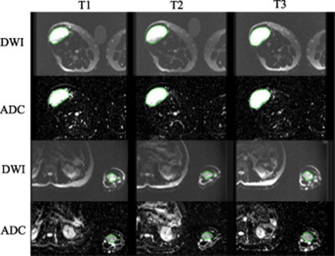
Figure 1. Example DWI images and ADC maps from sarcoma patients of the thigh (top two rows) and forearm (bottom two rows). Images acquired at the three time points (T1, T2, T3) were shown. Tumors were contoured in green. The bright cylindrical object outside the body was a tube phantom placed next to the patient for another study.
Download figure:
Standard image High-resolution imageBoxplots of mean ADC and delta ADC among the N0 and N1 groups were shown in figure 2. It is apparent that there was an overlap of the values between the two groups, and separating them using ADC or delta ADC alone was not feasible. This was confirmed by the low prediction AUC in figure 3. Overall, the performance using SVM model with only ADC as the feature was poor. The highest AUC was achieved using ADC_D31 (AUC = 0.69 ± 0.06).
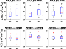
Figure 2. Boxplot of mean ADC and delta ADC among the two groups. P-value is from the unpaired t-test.
Download figure:
Standard image High-resolution image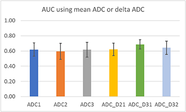
Figure 3. Prediction performance of SVM using only mean ADC or delta ADC.
Download figure:
Standard image High-resolution imageFigure 4 shows the model AUC with respect to the increasing number of features during the sequential forward selection process. For logistic regression, the AUC reached a maximum when three features were used in the model and decreased with four or more features, possibly due to overfitting. For SVM, the AUC reached a maximum near four features and then stabilized at an AUC of approximately 0.9. Therefore, three features were selected for logistic regression and four features were chosen for SVM. The three features selected by logistic regression were GLSZM Zone Entropy D31, GLCM Maximal Correlation Coefficient D31, and GLDM Large Dependence High Gray Level Emphasis D31. The top three features identified by SVM were the same as that of logistic regression. The fourth feature of SVM was GLDM Large Dependence Low Gray Level Emphasis D31.
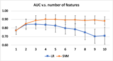
Figure 4. Model AUC with respect to different numbers of features from 1 to 10 for logistic regression and SVM. The error bar indicates the standard deviation. The best number of features 'k' was determined by inspecting the AUC curve. In this case, three features were identified for logistic regression and four features were selected for SVM.
Download figure:
Standard image High-resolution imagePrediction performance of logistic regression using the three selected features and SVM with the four selected features were shown in table 3. SVM significantly outperformed logistic regression for all statistics. An AUC of 0.91 and accuracy of 0.92 were achieved using SVM, while the AUC and accuracy were 0.85 and 0.87 for logistic regression.
Table 3. Prediction performance using all three time points and delta radiomics features.
| LR | SVM | |
|---|---|---|
| AUC | 0.85 ± 0.06 | 0.91 ± 0.05 |
| Sensitivity | 0.85 ± 0.07 | 0.90 ± 0.08 |
| Specificity | 0.94 ± 0.05 | 0.97 ± 0.04 |
| Accuracy | 0.87 ± 0.04 | 0.92 ± 0.04 |
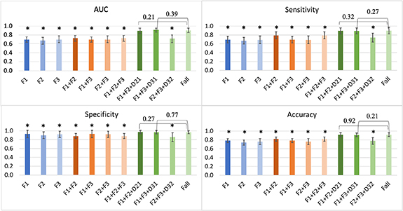
Comparisons of the SVM prediction performance using different time points and with/without delta radiomics features are shown in figure 5. Prediction performance using only a single time point was poor. AUC values for F1, F2, F3 were 0.70 ± 0.06, 0.67 ± 0.08, and 0.70 ± 0.08, respectively. Including a second or third time point without delta radiomics does not necessarily improve the prediction. AUC values for F1 + F2, F1 + F3, F2 + F3, and F1 + F2 + F3 were 0.70 ± 0.06, 0.73 ± 0.07, 0.70 ± 0.08, and 0.73 ± 0.07, respectively. Including delta radiomics D21 or D31 drastically boosted the prediction (AUC = 0.90 ± 0.06 for F1 + F2 + D21, and 0.91 ± 0.04 for F1 + F3 + D31), whereas D32 did not contribute much to improving the AUC (AUC = 0.72 ± 0.09). For all prediction statistics, there was no significant difference between Fall with F1 + F2 + D21 or F1 + F3 + D31.
Figure 5. Prediction performance using different time points. The error bar indicates the standard deviation. The star (*) implies a significant difference with the performance of Fall.
Download figure:
Standard image High-resolution image
Selected features for each of the models in figure 5 were summarized in table 4. It can be seen that as soon as delta radiomics were included in the feature pool, the majority of selected features were delta radiomics features. Among the 27 selected features, two belonged to the first-order feature, three belonged to the shape feature, nine belonged to the GLCM feature, eight belonged to the GLSZM feature, five belonged to the GLDM, and 0 were from the GLRLM or NGTDM categories.
Table 4. Selected features for models using features from different time points and with and without delta radiomics.
| Feature pool | Selected features |
|---|---|
| F1 | GLSZM Zone Entropy (F1), GLCM Maximal Correlation Coefficient (F1) |
| F2 | GLCM Cluster Shade (F2) |
| F3 | GLCM Cluster Shade (F3) |
| F1 + F2 | GLSZM Zone Entropy (F1), Shape Elongation (F2) |
| F1 + F3 | GLSZM Zone Entropy (F1), GLCM Maximal Correlation Coefficient (F1) |
| F2 + F3 | GLCM Cluster Shade (F3), GLCM Difference Variance (F2) |
| F1 + F2 + F3 | GLSZM Zone Entropy (F1), Shape Elongation (F2) |
| F1 + F2 + D21 | GLCM Maximum Probability (D21), First Order Skewness (D21), GLSZM Gray Level Variance (D21), First Order Median (D21), GLSZM Gray Level Nonuniformity Normalized (F1) |
| F1 + F3 + D31 | GLSZM Zone Entropy (D31), GLCM Maximal Correlation Coefficient (D31), GLDM Large Dependence High Gray Level Emphasis (D31), GLDM Large Dependence Low Gray Level Emphasis (D31), Shape Maximum 2D Diameter (D31) |
| F2 + F3 + D32 | GLDM Large Dependence Low Gray Level Emphasis (D32) |
| Fall | GLSZM Zone Entropy (D31), GLCM Maximal Correlation Coefficient (D31), GLDM Large Dependence High Gray Level Emphasis (D31), GLDM Large Dependence Low Gray Level Emphasis (D31) |
4. Discussion
Magnetic resonance imaging is a standard modality in the diagnosis and treatment planning of soft tissue sarcoma (Noebauer-Huhmann et al 2015). In addition to standard MRI sequences, DWI may provide additional information for characterizing soft tissue sarcoma at diagnosis (Rijswijk et al 2002, Schnapauff et al 2009, Lee et al 2016, Yoon et al 2019). In other tumor types, DWI has shown promise as a tool to assess treatment response (Byun et al 2002, Moffat et al 2004, 2005, Mardor et al 2004). However, there are limited data on the role of DWI in the assessment of treatment response in soft tissue sarcoma; the existing data in this field lean heavily on simple correlations between mean ADC or minimum ADC and patient outcome using one or two time points, without assessing other more complex predictive features or predictive models. In this proof of principle study, we showed the feasibility of predicting pathologic outcomes through functional imaging. We found that for our patient cohort, mean ADC or delta ADC alone did not reach a high prediction performance for treatment effect prediction. Radiomics features were needed to better capture tumor texture changes to improve the prediction. Despite the result still being preliminary, this study constitutes a very early step towards the ultimate goal of personalized patient management such as response-based radiation adaptation and radiation boosting for improved treatment efficacy, and non-operative management for patients with complete response to avoid potential surgical complications.
Establishing the optimal imaging acquisition timing during a radiotherapy treatment course is a critical step toward an efficient large-scale treatment response study trial. In this study, diffusion imaging was acquired three times throughout the five-fraction treatment. By comparing the prediction performance using different time points, it can be seen that information from a single or multiple time points alone was not sufficient to reflect the tumor's response to the treatment. It is crucial to include a change of feature to capture the tumor response to radiation. We found that after adding delta radiomics into the feature pool, the majority of selected features belong to delta radiomics (table 4), indicating changes of features are more predictive than static features. In addition, baseline information is needed for a good prediction. It needs be combined with either mid-treatment or post-treatment data to calculate the delta radiomics. Our results indicate that acquiring two imaging time points, either pre-treatment and mid-treatment, or pre-treatment and post-treatment, is sufficient for response prediction on our patient cohort.
For the model using all available features and delta features (Fall), three features were selected by both logistic regression and SVM: GLSZM Zone Entropy D31, GLCM Maximal Correlation Coefficient D31, and GLDM Large Dependence High Gray Level Emphasis D31. They measure the uncertainty/randomness in the distribution of zone sizes and gray levels, texture complexity, and the large dependency distribution of higher gray-level values, respectively (van Griethuysen et al 2017). This indicates that the changes in the complexity and distribution of ADC map are predictive of the radiotherapy response on sarcoma patient. All selected features belong to the D31 group, indicating the delta radiomics of pre-RT and post-RT is predictive of the TES.
The images of this study were acquired using the onboard MRI scanner of the ViewRay system. This MR-guided radiotherapy system made the longitudinal imaging acquisition throughout the treatment logistically practical. In addition, the large bore and flat table design of the system allowed the use of most conventional immobilization devices, so that the imaging could be reproduced for all following imaging sessions, to minimize signal variation caused by patient setup. However, the field strength of the MR scanner was 0.35 Tesla because of specific RT design goals (Raaijmakers et al 2008). Such a low magnetic field results in a relatively low image SNR, and the signal level of DWI approached the noise floor level at larger b values (Gao et al 2017). Therefore, the highest b-value used in this study was 500 mm2 s−1. The low SNR, poor spatial resolution, and lack of high b-value for diffusivity quantification could have a negative impact on extracting meaningful features. In this study, combined with the SVM model, the selected features provided a satisfactory prediction outcome. However, future study is warranted to investigate the effect of imaging protocol and field strength on feature calculation and model prediction.
Due to all patients being enrolled prospectively, at the time of compiling this study, other commonly used outcome evaluation criteria such as the development of metastases or long-term survival data were not available. TES was chosen in this proof-of-concept study for two reasons. First, as one direct impact of RT is cell-death, this radiation-induced pathologic treatment effect (which accounts for necrosis) intuitively reflects treatment efficacy. Second, although still controversial, several studies have shown the prognostic value of necrosis score (El-jabbour et al 1990, Hashimoto et al 1992, van Unnik et al 1993, Picci et al 1997, Bacci et al 2005). Therefore, accurate treatment effect predictions during or after RT but before the surgery could provide guidance for adjusting treatment strategies.
The main limitation of this work is the small patient cohort. Fifty-two patients were recruited to participate in the single-institution preoperative trial of hypofractionated radiotherapy from May 2016 to June 2018. Among them, 36 patients were enrolled in this longitudinal MRI study, and 30 patients had a full data set available for analysis. Repetitive cross-validation was applied to estimate the robustness. However, the results are potentially biased because we lack an independent test set. We are enrolling more patients on an expansion cohort to test the model and improve the model robustness. In addition, manual contouring is required for feature extraction, and this contouring process could introduce variability. Other classification models that do not rely on tumor segmentation, such as classifiers based on a conventional neural network (CNN), could be implemented for treatment effect prediction. However, compared with the SVM model, which works well for small patient numbers and provides explicit features for interpretation and clinically guidance, CNN-based classifiers usually require large amounts of training data and the trained model is hard to interpret. Lastly, although patients enrolled in this study each received the same treatment scheme, their histology subtypes are different. Sarcoma is known for its histologic and biologic diversity, and these differences are often reflected in divergent imaging characteristics. Myxoid liposarcoma, for example, which was well-represented in our study, has a unique MRI appearance. Ultimately, we aim to study patients based on histology category and analyze their response to treatment separately once a larger patient cohort is available.
5. Conclusion
Radiomics features from a longitudinal DWI were explored to predict the post-surgery tumor necrosis score after RT for sarcoma patients. The SVM model built with predictive radiomics features provided high prediction performance. Based on the observations of this study, we found that mean ADC, delta ADC, or radiomics features alone were not sufficient for response prediction. Delta radiomics features are needed to optimize radiomics prediction of the treatment effect on soft tissue sarcoma.
Acknowledgments
The authors would like to acknowledge the research support from ViewRay Inc.
Conflict of interest
The authors do not have any conflicts of interest to declare.