
Abstract
This study investigated the effect of temporal resolution on the dual-input pharmacokinetic (PK) modelling of dynamic contrast-enhanced MRI (DCE-MRI) data from normal volunteer livers and from patients with hepatocellular carcinoma. Eleven volunteers and five patients were examined at 3 T. Two sections, one optimized for the vascular input functions (VIF) and one for the tissue, were imaged within a single heart-beat (HB) using a saturation-recovery fast gradient echo sequence. The data was analysed using a dual-input single-compartment PK model. The VIFs and/or uptake curves were then temporally sub-sampled (at interval ▵t = [2–20] s) before being subject to the same PK analysis. Statistical comparisons of tumour and normal tissue PK parameter values using a 5% significance level gave rise to the same study results when temporally sub-sampling the VIFs to HB < ▵t <4 s. However, sub-sampling to ▵t > 4 s did adversely affect the statistical comparisons. Temporal sub-sampling of just the liver/tumour tissue uptake curves at ▵t ≤ 20 s, whilst using high temporal resolution VIFs, did not substantially affect PK parameter statistical comparisons. In conclusion, there is no practical advantage to be gained from acquiring very high temporal resolution hepatic DCE-MRI data. Instead the high temporal resolution could be usefully traded for increased spatial resolution or SNR.
Export citation and abstract BibTeX RIS
Introduction
This study investigated the effects of temporal resolution on the analysis of hepatic dynamic contrast-enhanced magnetic resonance imaging (DCE-MRI) data from volunteers and patients with hepatocellular carcinoma.
Dynamic contrast-enhanced magnetic resonance imaging is increasingly being used to evaluate the perfusion of organs and tumours, in the latter case potentially providing a biomarker for treatment response (Padhani and Leach 2005). Organ and tissue blood flow can be demonstrated qualitatively by the signal enhancement on T1-weighted images resulting from the uptake of an intravenously injected contrast agent. Quantitative measures of tissue perfusion and/or vessel wall permeability can be estimated by applying pharmacokinetic (PK) modelling to the contrast agent uptake curves following a bolus intravenous injection. This process ideally requires the measurement of the arterial input function (AIF) which is the concentration-time curve of contrast agent in the feeding artery.
The acquisition of DCE-MRI data from the liver is challenging for several reasons. Dynamically acquired images of the liver typically suffer from physiological motion related to breathing, cardiovascular pulsation and adjacent bowel motion. Additionally, the liver blood supply comprises two vessels, the hepatic artery and the portal vein. The first issue requires the application of motion correction or image registration algorithms. The second requires the modification of the Tofts PK model (Tofts and Kermode 1991) (or indeed most other PK models) to include a portal venous input function (PVIF) in addition to an AIF. When applied to the Tofts model the result is a dual-input single-compartment model which we will term the 'Materne model' (Materne et al 2000).
A possible limiting factor to such studies is the temporal resolution at which the vascular input functions (VIF) are acquired. This is because the first pass of the bolus lasts only a few seconds and commonly-quoted DCE parameters (such as the plasma fraction vp and the transfer constant Ktrans) are influenced by the shape and height of the AIF peak (Cheng 2008).
The temporal-sampling requirements for DCE-MRI data have previously been investigated largely in simulation and with the use of a variety of single-input compartmental models (Henderson et al 1998, Luypaert et al 2010, Lopata et al 2007, Di Giovanni et al 2010, Aerts et al 2011, Kershaw and Cheng 2010). Two other studies have used experimental data in pre-clinical and clinical settings, down-sampled by various means, to probe the effects of temporal resolution on resulting PK model parameters, again using single-input models (Heisen et al 2010, Larsson et al 2013). A further study (Michaely et al 2008) uses sub-sampling of experimental data in the context of renal DCE-MRI to conclude that a temporal resolution of at least 4 s is required for accurate measurement of plasma flow.
However in DCE-MRI studies of the liver involving the application of a dual-input model, there is little literature on temporal-sampling effects: Miyazaki et al (2008) analyse the errors involved in application of the Materne model to liver DCE-MRI data, though their discussion of temporal effects relates only to 'stretching' of the VIFs and not to the sampling strategy. Orton et al (2009) describe a comparison of two data acquisition protocols with temporal resolutions of 3.0 and 5.3 s.
The present study aimed to investigate these effects more systematically and employed temporal sub-sampling of high-temporal resolution experimental data from the livers of healthy volunteers and patients with hepatocellular carcinoma. These data were analysed using the Materne PK model.
Methods
Data acquisition
The study was approved by the local ethics review board and informed written consent was obtained from 11 healthy volunteers (9 male, 2 female) and from 11 patients (10 male, 1 female) with confirmed hepatocellular carcinoma (lesion <7 cm, median 3.5 cm, range 1.5–5.0 cm). Suitable subjects were approached consecutively. Diagnosis was by a combination of biopsy, imaging and/or raised alpha-foetoprotein level (AFP).
The subjects fasted for 8 h prior to the examination to ensure a base-line portal venous flow. Examinations were performed on a 3 T whole body MR system (Signa HDx, GE Healthcare, Waukesha, WI) using an 8-channel cardiac-array coil. The DCE series was collected using an ECG-triggered saturation-prepared fast gradient echo sequence modified with a saturation pulse train for improved B1 uniformity (Kim et al 2008, Oesingmann et al 2004). The saturation scheme was non-slice selective. Two images were acquired every heartbeat, for 512 heartbeats (Gatehouse et al 2004). Each image pair shared most acquisition parameters (matrix 128 × 128, parallel imaging acceleration (ASSET) factor 2, slice thickness 10 mm, TR/TE = 3.4/1.1 ms, NEX = 1, flip angle 10°, BW ± 31.2 kHz and centric phase ordering) but had individually specified saturation times and prescription geometry. ECG triggering was used to minimize the potential for any cardiac flow related artefacts.
Within each image acquisition pair in the dynamic series, the first sampled the two VIFs in an oblique orientation through the aorta and a cross section of the portal vein and employed a short saturation recovery time (TS = 20 ms) to minimize 'clipping' of the AIF (Gatehouse et al 2004). The second image was oriented sagittally through the liver and had a longer saturation recovery time (TS = 200 ms) to improve the SNR in the parenchymal images associated with lower contrast agent concentrations in tissue. The dynamic image set was acquired under conditions of free shallow breathing.
All subjects received an intravenous bolus injection of 0.1 ml kg−1 of 1.0 M gadobutrol (Gadovist, Bayer Schering, Germany) into an antecubital vein, administered at 6 ml s−1 followed by a 25 ml saline flush injected at the same rate, using a power injector (Spectris; Medrad, Indianola, PA). The injection was given after approximately 20 s of baseline imaging.
Image analysis
The dynamic series of images was analysed using custom software developed in MATLAB (The Mathworks, Natick, MA). Within the dynamic series and on the oblique slice set of images, regions of interest (ROI) were drawn manually just inside the lumen of the portal vein and aorta. Physiological motion of the portal vein throughout the image series was tracked automatically, and the ROI position updated by rigid body translation on each image. It was found that placement of the aortic ROI required no correction for physiological motion.
In both volunteers and patients, a further ROI was placed on the sagittal images in an area of the liver parenchyma with no visible vessels or disease present (see figure 1). In the patients, an additional ROI was drawn around the primary liver tumour image at a representative time point. Rigid translational motion correction was performed first automatically and then manually for fine adjustments. The automated process involved moving the ROI on successive images in step with the vertical position of the diaphragm. These preliminary ROI placements were then checked and adjusted manually, using rigid-body translation, for all images in the dynamic series.
Conversion of signal to [Gd]
The following relationships were used to convert the mean ROI tissue dynamic signal intensities (SI) to contrast agent concentrations, [Gd]. Equation (1) is the standard saturation-recovery signal relationship:

where SITS→∞ is a normalization factor equal to the signal obtained using a very long saturation recovery time. [Gd] is then calculated from T1 and T10 using the standard relaxivity relationship:

Here, T10 is the pre-contrast T1 of the tissue or blood, r is the relaxivity of the contrast agent (4.5 s−1 M−1 for gadobutrol at 3 T (Pintaske et al 2006)). Substituting for T1 and T10, which may be obtained from the pre-contrast base-line signal SI0 by substitution in equation (1), we have:

SITS→∞ was measured, using the same ROIs placed on the dynamic series, as the signal from a single independent acquisition of the saturation prepared FGRE pulse sequence after a very long saturation recovery time (in practice after TS = 10 s). This acquisition was made before the administration of contrast agent. SI0 was measured as the mean of the first ten base-line signals obtained from the dynamic series before the point of administration of contrast agent (neglecting the first time-point).
Blood Gd concentrations were converted to plasma concentrations using an assumed hematocrit of 0.45.
Sub-sampling of data
In order to investigate the effects of temporal resolution, the acquired VIF [Gd] curves were sub-sampled by linear interpolation with a sampling interval of ▵t = 2–20 s, at 1 s increments. The temporal offset for sub-sampling was varied from 0–▵t s at 1 s increments and nested inside the ▵t variation, so that effects of temporal jitter could be averaged across the subsequent set of results. The tissue Gd uptake curve was sub-sampled to the same temporal resolution as the VIFs in each case.
The high injection rate (6 ml s−1) was chosen to give a narrow AIF peak and hence generate a worst-case AIF form for sub-sampling.
An additional sub-sampling regime was also implemented in which only the tissue Gd uptake curve was sub-sampled leaving the VIFs at their original high-temporal resolution. This was to emulate the hypothetical case of the VIFs being acquired from a pre-bolus injection (Kershaw and Cheng 2011).
Pharmacokinetic modelling
The mean plasma Gd concentration time courses, Ca(t) and Cp(t), were extracted from the aorta and portal vein ROIs. The liver tissue concentration time course CL(t) was also extracted, derived from the mean MR signal from the whole ROI. These were fitted (using non-linear least-squares optimization) to the Materne PK model (Materne et al 2000) to yield five parameters: transfer constants k1a and k1p, rate constant k2, and circulation delays τa and τp:

The circulation delay τa represents the (unknown) time taken for blood to flow from the site of measurement of the AIF to the capillary bed in the tissue of note. The time delay τp is similarly defined with respect to the portal vein and the capillary bed.
Equation (4) can be integrated to yield the following solution for CL:

Curve-fitting to this equation was carried out using the MATLAB Optimisation Toolbox function 'lsqcurvefit()' which employed a trust-region reflective algorithm (Coleman and Li 1996) and used the default convergence criteria (100 iterations, tolerance 10−6). All five free parameters were fitted using this gradient-descent method. No constraints were imposed except for the requirement that the circulation delays, τa and τp, should be between (0–10) s. Integrals in the curve-fitting function were performed using trapezoidal numerical integration, the step-size being determined by the temporal sampling rate of the original VIFs. Down-sampled curves were re-sampled to this higher temporal resolution by linear interpolation for the purposes of integration.
To avoid convergence of the fitting process on a local minimum, the curve fitting process was repeated for a set of 8 starting values K0i = (k1a0, k1p0, k20, τa0, τp0)i taken from a physiologically realistic range for each of the first three parameters and set at zero for each of the circulation delays, i.e. (0.000–0.003 s−1, 0.000–0.030 s−1, 0.000–0.120 s−1, 0 s, 0 s). The best-fitting solution, judged on the basis of the residual squared norm, was accepted.
To check the validity of using the 5-parameter model, a 3-parameter model nested within it by fixing τa = τp = 0 s (following the work of other researchers e.g. (Miyazaki et al 2008)) was also fitted to the high temporal-resolution data.
Using the derivations and naming conventions of references (Tofts et al 1999, Materne et al 2002) the following quantities were calculated from the fitted model parameters k1a, k1p and k2 (s−1): total plasma flow, F = 6000.(k1a + k1p) (ml/min/100 ml); arterial fraction, A = 100.k1a/(k1a + k1p) (%); mean transit time, MTT = 1/k2 (s); and distribution volume, D = 100.(k1a + k1p)/k2 (%).
Statistical comparisons between tumour and normal volunteer parameters were carried out using the Mann–Whitney U-test (performed using the MATLAB Statistics Toolbox). The validity of using a 5-parameter curve-fit as opposed to the 3-parameter fit nested within it was investigated using an F-test (see, for example, (Glatting et al 2007)).
Results
Due to operator error two patients' examinations did not did not yield data suitable for PK model analysis. A further patient examination failed due to technical problems with the acquisition. The remaining 8 patient data-sets were analysed along with the 11 volunteer data-sets. A further patient data-set was then rejected because inaccurate ECG triggering had resulted in the temporal resolution becoming twice the R–R interval; a further two patient data-sets were rejected because of poor fitting of the data to the Materne model. Results are therefore quoted for 5 patient data-sets and 11 volunteer data-sets. Sample VIFs for one volunteer, the tissue uptake curve and the model fit are shown in figure 1.
The results from the 3-parameter fit on the original high-temporal resolution data were similar but not identical to those from the 5-parameter fit. The F-test comparing the 3 and 5-parameter fits showed a statistically significant result (P < 0.05) in 17/21 cases (17/21 cases = 8/11 volunteer curve-fits +5/5 background liver curve-fits +4/5 tumour curve-fits). This justified the use of the more complex model to fit this data.
Table 1 shows the volunteer PK model parameter results from the current study (using the original high temporal resolution data) compared with similar studies carried out by other researchers (Hagiwara et al 2008, Baxter et al 2009, Patel et al 2010).
Table 1. Perfusion parameter results (mean ± SD) from normal volunteers in this study compared with recent published studies. (Note that whole blood flow, Fb, is quoted in this table rather than plasma flow: the relationship Fb = F/(1 – Hct) is assumed, with the hematocrit Hct = 0.45.) P-values (from Student t-tests) refer to the null hypothesis that the difference in the parameter mean in question between the present study and the compared study is zero (significant values at 5% level shown only).
| Study | N | Fb (ml/min/ 100 ml) | A (%) | MTT (s) | D (%) | τa (s) | τp (s) |
|---|---|---|---|---|---|---|---|
| Hagiwara | 10 | 138 ± 69 | 7.5 ± 7.9 | 9.3 ± 4.3 | 17.3 ± 3.9 | Not | Fixed at |
| 2008 | reported | zero | |||||
| Baxter | 35 | 148 ± 49 | 18.7 ± 4.4 | 7.5 ± 1.5* | 14.0 ± 4.2 | Not | Not |
| 2009 | (P < 0.001) | reported | reported | ||||
| Patel 2010 | 6 | 133 ± 82 | 16.3 ± 3.3 | 17.4 ± 15.4 | 23.9 ± 8.4* | Not | Fixed at |
| (P = 0.022) | reported | zero | |||||
| This study | 11 | 142 ± 116 | 15 ± 21 | 17 ± 12 | 15 ± 6 | 3.2 ± 3.6 | 3.4 ± 3.3 |
Table 2 shows the P-values yielded by the statistical tests (Mann–Whitney) carried out on the parameter values in tumours in comparison with those in healthy volunteer livers (with the null hypothesis that there was zero difference in means).
Table 2. P-values from the Mann–Whitney U-test of the null hypothesis of no difference between parameter means from normal volunteer liver tissue and HCC tumours in patients. This is shown for the high-temporal resolution data-set and data-sets created by subsequent temporal re-sampling at ▵t = 4, 10 and 20 s. Two cases are shown: (a) sub-sampling of all curves (VIFs and tissue uptake) and (b) sub-sampling of just the tissue uptake curve.
| (a) VIFs and tissue curve sub-sampled | (b) Tissue curve only sub-sampled | |||||||
|---|---|---|---|---|---|---|---|---|
| P-value ▵t (s) | F | A | MTT | D | F | A | MTT | D |
| Heart-beat | 0.002* | 0.001* | 0.001* | 0.267 | 0.002* | 0.001* | 0.001* | 0.267 |
| temporal | ||||||||
| resolution | ||||||||
| 4 | 0.052 | 0.003* | 0.002* | 0.510 | 0.002* | 0.002* | 0.001* | 0.267 |
| 10 | 0.115 | 0.002* | 0.009* | 0.743 | 0.001* | 0.002* | 0.001* | 0.320 |
| 20 | 0.743 | 0.001* | 0.003* | 0.510 | 0.002* | 0.002* | 0.003* | 0.261 |
Figure 2 shows sample VIFs and their down-sampled counter-parts, with ▵t = 4 s. Figure 3 shows the consequences of temporal sub-sampling in the 11 volunteers, the 5 background liver regions in patients and the 5 HCC tumours. The PK parameter results are shown from the original high temporal resolution data, and those from the same curves (uptake and VIFs) sub-sampled to ▵t = 4 s and those from ▵t = 20 s. There is little difference between results from the high-temporal resolution data and those sampled at 4 s; on the other hand there are appreciable differences at ▵t = 20 s.
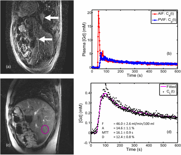
Figure 1. Example of high temporal resolution VIFs and uptake curve measured in a volunteer: (a) dynamic series image (first in pair) with upper arrow marking the aorta and lower arrow marking the portal vein; (b) extracted VIFs (plasma Gd concentration); (c) dynamic series image (second in pair) showing normal liver ROI placed in an area devoid of major vasculature; (d) the uptake curve together with the curve fitted by the Materne model and the fitted parameter values.
Download figure:
Standard image High-resolution image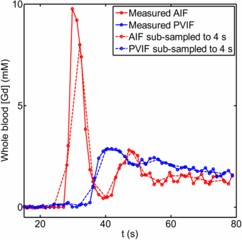
Figure 2. Example of VIFs (whole blood Gd concentrations) measured in a volunteer and their sub-sampled counterparts (interval 4 s): (solid red line) arterial input function; (solid blue line) portal venous input function; (dashed red line) sub-sampled arterial input function; (dashed blue line) sub-sampled portal venous input function. (First 80 s of data only shown here.)
Download figure:
Standard image High-resolution image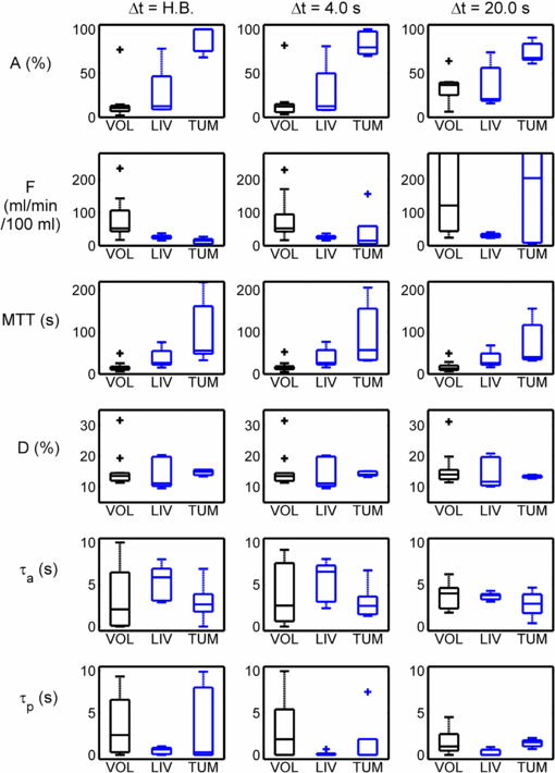
Figure 3. Physiological parameters derived from the results of PK modelling applied to the uptake curves and VIFs: (left) analysis applied to high-temporal resolution (heart-beat) data; (centre) analysis applied to the same data with all VIF and tissue curves sub-sampled to a temporal resolution of 4 s; (right) analysis applied to the same data, sub-sampled to a temporal resolution of 20 s.
Download figure:
Standard image High-resolution imageThe plots in figure 4 show the bias associated with each parameter at varying sub-sampling intervals, where the bias is defined as the mean difference between paired measurements of the selected parameter at high-temporal resolution and at the ▵t under consideration. The plots in figure 5 show the bias along with the 95% confidence interval of the differences between paired measurements of the selected parameter. (Put more simply, these graphs show at each ▵t the bias and 95% confidence interval which would be displayed on a Bland–Altman plot of the ▵t measurements concerned when compared against the high-temporal resolution measurements serving as 'gold standard'.)
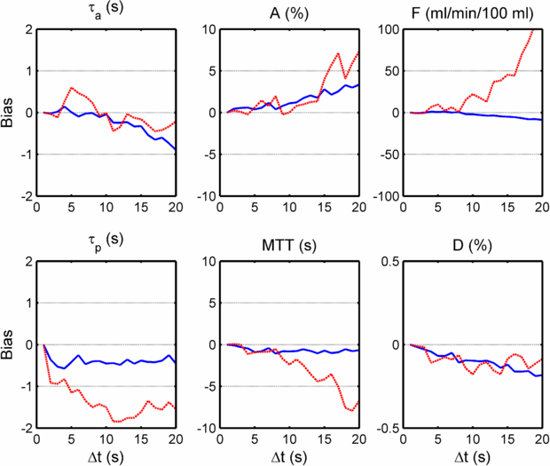
Figure 4. Plots of the bias observed in each model parameter at a temporal resolution of ▵t = 2–20 s, when compared with a 'gold-standard' consisting of the results from the high-temporal resolution data (volunteer and patient data combined). In each, two cases are shown corresponding to the temporal sub-sampling of the VIFs and uptake curves (dotted red lines) and the same with only the tissue uptake curves sub-sampled (full blue lines).
Download figure:
Standard image High-resolution image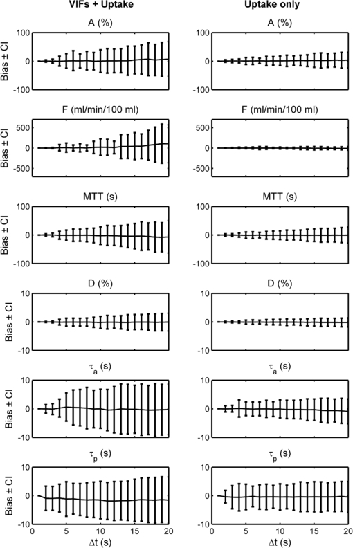
Figure 5. As figure 4 but showing the 95% confidence interval on the bias in addition to the bias itself: (left) VIFs and uptake curves both sub-sampled; (right) only the tissue curve sub-sampled. The bias is as compared to the high temporal resolution analysis acting as 'gold-standard'.
Download figure:
Standard image High-resolution image
Figures 4 and 5 also show similar results for the case of temporal sub-sampling of the tissue uptake curves only (i.e. using the high-temporal VIFs in all cases).
Discussion
A method has been described for acquiring high temporal resolution VIFs and single slice DCE-MRI data in the liver of human subjects at 3 T, using a dual-acquisition saturation-prepared fast gradient echo pulse sequence. Temporal sub-sampling of the data curves was carried out to yield information about the dependence of the Materne dual-input single compartment PK model parameters on the sampling interval.
The high temporal resolution data from volunteers produced results which are in line with, although slightly more variable than those found in the literature from studies at 1.5 T, using a variety of MR imaging techniques (Hagiwara et al 2008, Baxter et al 2009, Patel et al 2010) (see table 1). The high variability in our data could be due to genuine heterogeneity in the patient sample or alternatively to reduced precision in measurement. The present study employed different motion correction and curve-fitting techniques compared to the other studies cited. However, in the absence of repeatability data it is difficult to conclude that these are the cause of the high variability observed.
The plots of bias and 95% confidence interval over all curves sub-sampled (see figures 4 and 5) show a gradual deterioration of accuracy and precision in parameter values (with respect to the high temporal resolution 'gold-standard') with increasing ▵t. In particular, plasma flow (F) is over-estimated with increasing ▵t. Although the dual vascular input to the liver complicates the picture, this finding may be contrary to the conclusion of Larsson et al (2013), who found that in gliomas the Ktrans parameter in the extended Tofts models is under-estimated with increasing ▵t. (The transfer constants k1a and k1p, and hence the derived parameter F, in the Materne model fulfil a similar role to Ktrans in the Tofts model. However, it should be noted that the extended Tofts model is based on two compartments which makes the comparison with the Materne model even less straightforward.) Larsson does, however, report a transient increase in Ktrans for ▵t <20 s (if the MTT is relatively long). Aerts et al (2011) found that the Ktrans estimated in simulations using the extended Tofts model and the Parker population average AIF (Parker et al 2006) was over-estimated with increasing ▵t, which supports our findings.
In our study, the arterial fraction, A, is over-estimated as ▵t increases: this can be understood in terms of the greater effect of sub-sampling on the AIF peak as opposed to the PVIF peak (see figure 2). This in turn would act to increase k1a more than k1p as ▵t is increased.
The fact that the distribution volume D is relatively robust to changes in temporal sampling partially supports the findings of Heisen et al (2010) and Di Giovanni et al (2010) who reported that the analogous parameter using the Tofts model (ve) measured in breast tumours was stable throughout a change in ▵t from 10–70 s.
It is instructive to gauge the effect of these results on typical study conclusions. A commonly quoted result in hepatic DCE-MRI is the difference between parameter values in tumours as opposed to those in normal healthy livers. The P-values shown in table 2 indicate that, at least for our sample of 5 patients and 11 volunteers, sub-sampling all curves to 4 s makes very little difference to the statistical significance of comparisons at the 5% level. (The P-value of 0.052 for plasma flow is approximately at the limit for 5% significance.) Further sub-sampling to 10–20 s substantially changes the significance level for F. The 4 s cut-off is of course somewhat arbitrary since a lower value would be obtained if a 1% significance level was chosen. However, since the 5% level is commonly applied to DCE-MRI parameter comparisons in similar studies, the 4 s threshold serves as a reasonable guide.
The situation is more straightforward with sub-sampling only the tissue curve: here significances are not changed even when sub-sampling to 20 s. Other authors have reported on the efficacy of pre-bolus methods in DCE-MRI (Li et al 2012) and our results would support the use of high temporal resolution pre-bolus methods in hepatic studies whereby the tissue and VIF curves are sampled at different rates. In practice, however, at long ▵t there can be imaging artefacts associated with respiratory motion unless breath-holding techniques can be employed. It should also be noted that these comparisons take account of the bias created by sub-sampling and not the variance, which can be seen to be substantial (see figure 5).
The finding of Michaely et al (2008) that plasma flow from a two compartment model of renal function is accurately reported only if a temporal resolution of <4 s is employed, is in marked agreement with our own findings. Given the substantial differences in anatomical setting and the models employed to describe it, this may indicate that the limiting factor in each study is the temporal resolution required to accurately capture the AIF. This is supported by our results from the sub-sampling of the tissue curve only.
There are some acknowledged limitations of this study. A more sophisticated approach could have been applied to the temporal sub-sampling process: other researchers have adopted an approach based on averaging successive image data before extracting the signal curves (Larsson et al 2013) or on simulating the k-space of intermediate image data (Heisen et al 2010). It is doubtful whether these techniques would have made a significant difference to our study results since the effects are acknowledged to be small. Temporal jitter could have been applied separately for the VIFs and the tissue curve, as a situation in which these are sampled from different acquisitions is foreseeable. However, for simplicity and since temporal jitter will in any case have minimal effects on the tissue curve at the values of ▵t sampled, we made no assumption of temporal independence.
The Materne model has previously been shown to be adequate for healthy liver tissue although possibly not in liver tumours which have an almost exclusively arterial blood supply (Banerji et al 2012). In our study, however, the Materne model fitted tolerably well to the tumour data retained and returned a high arterial fraction as expected. As mentioned above, the patient data not fitted well by the model were excluded from the statistical analyses. (It should be noted that in the two cases where the tumour data was poorly fitted by the Materne model, the background liver tissue data was also not well fitted: this raises the possibility of another systematic error in these particular patient analyses as well as or instead of the model not being suitable.)
The high temporal resolution data acquired in this study allows independent estimation of the circulation delays, τa and τp; as expected, these parameters become less well defined as ▵t is increased. Though the F-test results support use of the 5-parameter model on the high temporal resolution data, it is debatable whether a 5-parameter fitting process is still appropriate at larger values of ▵t. However, for reasons of consistency, and since τa and τp are true unknowns with an assumed value potentially also leading to systematic error, the 5-parameter model was adopted for use on all patient and volunteer data. Our high temporal resolution data results give mean values for the circulation delays which are approximately equal (τa = 3.2 ± 3.6 s and τp = 3.4 ± 3.3 s). Intuitively one might expect a longer venous than arterial delay although this does in fact remain un-verified in the literature.
We have not included simulated data in this study because it is not yet possible to adequately model a representative PVIF. Much work has been done on the simulation of AIFs (for example, see Parker et al (2006)) but there is little similar literature for the PVIF. Banerji et al (2012) make a reasoned attempt though there are debatable assumptions involved in the process. For these reasons, we chose to sub-sample experimental data.
The authors note that other liver tumour types (as distinct from hepatocellular carcinoma) which have higher rates of contrast agent uptake, may require the sampling of higher temporal resolution data (i.e. ▵t < 4 s) in order to be adequately characterized.
Conclusion
This study shows that there is a continuous degradation of accuracy and precision of hepatic DCE-MRI parameters derived from a dual-input single-compartment model applied to high temporal-resolution experimental data when subjected to temporal sub-sampling. However, typical statistical comparisons at the 5% level between HCC tumour and healthy liver parameter results show no difference in significance when sampling the VIFs and tissue curves at intervals ▵t ≤ 4 s. When sub-sampling just the tissue curve, this interval could be as large as 20 s without affecting statistical significances.
These results imply that the gains in acquiring DCE-MRI data in the liver at increasingly high temporal resolution may be minimal. This has implications for more typical 3D acquisitions of DCE-MRI data in the liver which cannot be performed at very high temporal resolution without severely compromising image quality through SNR reduction.
Acknowledgments
The authors wish to thank Lorenzo Mannelli and Peter Beddy for assistance with establishing the study and for initial patient recruitment. We also thank Ilse Patterson and the MRIS radiographers for assistance with MR examinations, and the NIHR Cambridge Biomedical Research Centre, Cambridge Experimental Cancer Medicine Centre, Addenbrooke's Charitable Trust and Cancer Research UK for funding support.