

Abstract
Gas flaring during oil extraction over the Arctic region is the primary source of warming-inducing aerosols (e.g. black carbon (BC)) with a strong potential to affect regional climate change. Despite continual BC emissions near the Arctic Ocean via gas flaring, the climatic impact of BC related to gas flaring remains uncertain. Here, we present simulations of potential gas flaring using an earth system model with comprehensive aerosol physics to show that increases in BC from gas flaring can potentially explain a significant fraction of Arctic warming. BC emissions from gas flaring over high latitudes contribute to locally confined warming over the source region, especially during the Arctic spring through BC-induced local albedo reduction. This local warming invokes remote and temporally lagging sea-ice melting feedback processes over the Arctic Ocean during winter. Our findings imply that a regional change in anthropogenic aerosol forcing is capable of changing Arctic temperatures in regions far from the aerosol source via time-lagged, sea-ice-related Arctic physical processes. We suggest that both energy consumption and production processes can increase Arctic warming.
Export citation and abstract BibTeX RIS

Original content from this work may be used under the terms of the Creative Commons Attribution 3.0 licence. Any further distribution of this work must maintain attribution to the author(s) and the title of the work, journal citation and DOI.
1. Introduction
In addition to major global oil reservoirs, such as those in the Middle East and United States, huge amounts of untapped oil lie in Arctic regions (Gautier et al 2009). With increasing accessibility to such previously frozen territory due to dramatic warming of the Arctic region during the last several decades (Serreze et al 2009), major oil companies are continuously looking to exploit oil reservoirs in the far north (Howard 2009, Harsem et al 2011). Studies on oil extraction over Arctic regions have clearly shown strong environmental impact related to gas flaring from oil extraction (Ødemark et al 2012, Stohl et al 2013, Sand et al 2016). Gas flaring is a conventional method for disposing of gaseous and liquid hydrocarbons through combustion at oil/gas production and processing sites due to a lack of pipelines and other gas transportation infrastructure, as well as for protection against the dangers of over-pressurizing industrial plant equipment (Huang and Fu 2016; hereafter HF16). From the perspective of climate change, particulate matter from gas flaring predominantly takes the form of black carbon (BC) (HF16), which has a strong potential to change the degree of Arctic warming through the absorption of solar radiation, which will subsequently heat the atmosphere (Ramanathan and Carmichael 2008, Bond et al 2013), while also reducing albedo when deposited on snow and ice (Flanner et al 2007, 2009, Hadley and Kirchstetter 2012, Stohl et al 2013). Furthermore, due to the potential of future increasing trends in oil extraction (Peters et al 2011) in regions with melting sea ice, gas-flaring-induced BC emissions could increase more than expected.
However, our understanding of the climatic impact of gas-flaring-derived BC on the Arctic climate remains limited. Moreover, most emission inventories, including that in the Intergovernmental Panel on Climate Change (IPCC)'s Fifth Assessment Report (AR5, Stocker et al 2013) (see supplementary figure S1(a), which is available online at stacks.iop.org/ERL/14/094011/mmedia based on the emission inventory of the AR5), have neglected BC emissions from gas flaring. Therefore, quantitative assessment of the impact of gas-flaring-derived BC on the Arctic climate is necessary to understand the present Arctic climate and future global climate projections. In this study, we first investigated the response of the Arctic climate to gas-flaring-related BC emissions through sensitivity experiments using a numerical model.
2. Gas-flaring BC in satellite data
Gas-flaring activities can be detected using night-time light (NTL) data measured from space-borne systems. For instance, NTL data from the DMSP-OLS (Defense Meteorological Satellite Program/Operation Line Scanner) are frequently used for the monitoring of urbanization extent (Huang et al 2014), forest fires (Cahoon et al 1992) and gas flaring (Croft 1973). We used average visible stable lights, a product from NTLs of DMSP/OLS provided by NOAA (available online at https://ngdc.noaa.gov/eog/dmsp/downloadV4composites.html). The NTL product is retrieved from the average visible band digital number (DN). DN represents the units of nightlight observations and ranges from 0–63 corresponding to the observed brightness of the object. We note that DN is not perfectly proportional to the physical amount of light emitted, since the ephemeral lights and background noise are removed from the stable light product (Henderson et al 2012, Elvidge et al 2014). As a preliminary inquiry, we calculated the difference in NTL brightness between periods of economic decline (1990s) and growth (2000s) in Russia (figure 1). The overall frequency and extent of NTL brightness increased across many areas of Russia over time, in particular in the Khanty-Mansiysk and Yamalo-Nenets regions, the main oil and gas production fields in Russia. Given that Russia dominates the global gas-flaring BC emissions, accounting for an overwhelming fraction of about 57% (HF16), the increase in frequency and brightness of NTL presents strong evidence for enhanced gas-flaring activity during the recent period of economic growth in the 2000s.

Figure 1. ΔDN stands for differences in DN of NTL brightness from the DMSP/OLS satellite between the 1990s and 2000s. Positive (red) values denote an increase in brightness over time and negative (blue) values represent a decrease over time. NTL signals from urban centers and surrounding regions are masked in this figure.
Download figure:
Standard image High-resolution image3. Methods
3.1. Model
Effects of flaring-related BC over the northern high-latitude region were diagnosed from simulations of the National Center for Atmospheric Research CESM ver. 1.2 (Vertenstein et al 2013), consisting of the Community Atmospheric Model 5 (CAM5) coupled with the Community Land Model 4, sea-ice model CICE4 and a Slab Ocean Model (SOM) that facilitates fast equilibration. CAM5 offers more sophisticated aerosol mixing, aerosol–cloud interactions and aerosol deposition (Liu et al 2012) and simulates reasonably well the magnitude of BC in snow concentration against the measurements (Qian et al 2014). Furthermore, CESM1 simulates transient changes in Arctic surface temperature and sea-ice extent relatively well (Meehl et al 2013).
3.2. Experiments
To examine the influence of an increase in BC surface emissions, we conducted two runs: a control run (CONT) using the Intergovernmental Panel on Climate Change (IPCC)'s Fifth Assessment Report surface BC emissions (Lamarque et al 2010; supplementary figure S1(a)), and a sensitivity run (FLARE) with additional observed flaring-related BC over the Arctic region (supplementary figure S1(b)). Except for the BC emission input, all components, including present-day CO2 concentrations (367 ppmv), were the same in the CONT and FLARE runs. The atmospheric conditions were prescribed according to the monthly climatology of 1982–2001. Time-slice (equilibrium) experiments have the advantage of providing a large statistical sample of the changing climate (Cubasch et al 1995). The experiments were run for 230 years, and the last 200 years was used to assess the model response to BC emission changes in an equilibrium state. A two-tailed student's t-test was performed to determine the significance of differences in the means between CONT and FLARE.
In addition, we conducted the same experiment using only the atmospheric model not coupled with the ocean model to investigate the role of the ocean and related sea ice. A_FLARE (A_CONT) had the same conditions as FLARE (CONT), except for the prescribed sea surface temperature and sea-ice extent.
3.3. Flaring-related BC emission data
We used an average gas-flaring-related BC emission rate (HF16, supplementary figure S1(b); available online at https://www.nature.com/articles/sdata2016104) over only high-latitude northern regions above 60°N for the equilibrium model run. In HF16, gas-flaring-related BC emission rates were estimated from an emission factor database and flaring volumes retrieved from satellite imagery. Furthermore, the data set was compared against the absorption aerosol optical depth obtained from the MISR (multiangle imaging spectroradiometer) in Russia's gas-flaring source regions and ground-based BC measurements in Svalbard (see figures 3 and 4 in HF16). The BC emissions in Arctic regions north of 60°N were 19 Gg yr−1 in CONT and 80 Gg yr−1 in FLARE. All other emission inventories were from the IPCC (Lamarque et al 2010). Recently, the ECLIPSE (evaluating the climate and air quality impacts of short-lived pollutants) emission inventory has considered gas-flaring-related BC emissions (Stohl et al 2015).
4. Results
4.1. Local responses during spring
Figure 2(d) presents the monthly difference in surface air temperature (SAT) between the two experimental runs (FLARE—CONT) over the West Siberian petroleum basin shown in figure 1. The warming response was greatest during spring (March to May), consistent with previous findings (Flanner et al 2009) that near-surface BC induces extreme Arctic warming. Although combustion of gaseous and liquid hydrocarbons for their disposal did not vary seasonally (HF16), the response to increased levels of BC was most robust in spring (figure 2(d)). Figure 2(a) shows the changes in spring SAT poleward of 50°N. As expected, warming was most noticeable in areas with additional flaring-related BC emissions. Significant warming was also observed over the Atlantic and the Chukchi Sea. However, vertical penetration of warming was limited, because the strongly stratified mean vertical temperature profile in the Arctic (Hansen and Rosen 1984, Hansen and Novakov 1989) limited vertical mixing (figure 2(c)). By contrast, warming induced by BC transported from mid-latitudes occurs in the mid-troposphere (Sand et al 2013). Furthermore, the results confirmed that increased BC concentrations were limited to 900 hPa and below (not shown).
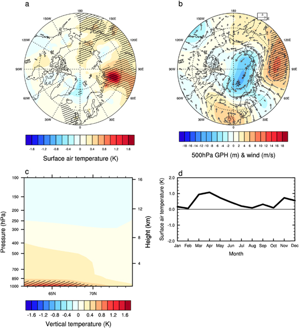
Figure 2. (a) Response of SAT to updated flaring-related BC during spring. (b) Responses of geopotential height (GPH) and wind at 500 hPa. (c) Vertical structure of the temperature response, as defined by the green box in (b) (60°–90°E, 60°–75°N). (d) Monthly response of SAT to updated flaring-related BC, as defined by the green box in (b) (60°–90°E, 60°–75°N). Hatched regions in (b)–(d) indicate significant differences at the 95% confidence level.
Download figure:
Standard image High-resolution imageChanges in the amount of BC aerosols can modify the surface energy budget through the direct effects of additional aerosols. The response of individual terms in the area-averaged surface energy budget is summarized in table 1. The dominant response in spring was an increase in net shortwave (SW) radiation (4.9 W m−2) at the surface. The surface energy budget indicated that surface fluxes and longwave (LW) radiation compensated for the absorbed SW radiation at the surface. This substantial increase in net SW radiation at the surface was associated with a reduced albedo (−4%; figure 3(a)). Note that the Snow Ice and Aerosol Radiation model (Lawrence et al 2011) in the Community Land Model used in this study effectively captures the effect of aerosol deposition (e.g. black and organic carbon and dust) on albedo (Hadley and Kirchstetter 2012).
Table 1. Surface energy changes according to flaring-related BC emissions over the forcing region.
| Variables (W m−2) | Spring | Summer | Autumn | Winter |
|---|---|---|---|---|
| Net SW radiation | 4.9 | 1.5 | −0.2 | 0.1 |
| Net LW radiation | 1.0 | 0.7 | −0.2 | −0.1 |
| Latent heat | 1.5 | 1.2 | 0.3 | 0.0 |
| Sensible heat | 1.2 | 0.5 | −0.1 | 0.1 |
Note: Bold font indicates statistical significance at the 95% confidence level.
Because BC is an aerosol that strongly absorbs solar radiation (Bond et al 2013), we assumed that a greater amount of solar radiation would induce a stronger response. However, solar radiation is greatest in summer. Therefore, the maximum warming responses in spring were likely linked to the observed surface albedo changes, which contributed to the most pronounced response in spring. The climatological spring surface albedo over the flaring-related BC area ranged from 40%– 70%, and the surface albedo difference due to additional BC from gas flaring reached −20% over the region (figure 3(a)). This value fell within the albedo reduction values of BC-laden snow observed in a laboratory experiment (Hadley and Kirchstetter 2012). Such reductions in surface albedo were mainly driven by BC deposition (figure 3(b)), due to the darkening of white snow-covered surfaces. Because the amount of increased flaring-derived BC was constant throughout the year in the model, the amount and distribution of total deposition remained very similar among the seasons (not shown). However, the response exhibited seasonal variation due to changes in background albedo. That is, in spring, the albedo effect is most significant because the area is covered with snow. Although BC is also deposited on the surface in summer, the snow-albedo effect is insignificant in seasons with relatively little snow cover (figure 3(c)). By contrast, because insolation is low (<100 W m−2) during October to February (i.e. the cold season; see the black line in figure 3(c)), the albedo effect due to deposited BC is negligible.

Figure 3. Responses of (a) albedo and (b) total (dry + wet) deposition rate of BC to updated flaring-related BC emissions during boreal spring. (c) Climatological seasonal cycle of insolation (black) and responses of snow depth (red) and albedo (blue) to updated flaring over the West Siberian petroleum basin. Hatched regions in (a) and (b) indicate significant differences at the 95% confidence level.
Download figure:
Standard image High-resolution imageCirculation changes caused by updated flaring-related BC emissions were investigated by examining changes in GPH at 500 hPa (figure 2(b)). There was an anomalous negative pressure center over the Arctic Ocean north of 70°N, while positive pressure anomalies were found over the circumpolar regions. This Arctic low-pressure/circumpolar high-pressure pattern caused the wind to blow from the West Siberian petroleum basin to the Arctic Ocean. Interestingly, the changes in the circulation filed due to the gas-flaring BC show similar circulation structures to the previous studies, which revealed the relationship between Arctic warming and the associated poleward moisture transport (Luo et al 2017, Zhong et al 2018). The poleward moisture transport results in an increase in downward longwave radiation (DLR) inducing warming near the Barents-Kara Seas (Woods and Caballero 2016, Luo et al 2017, Zhong et al 2018).
4.2. Remote and lagged responses
Figure 4 shows the monthly mean difference in SAT over the Arctic Ocean. While the warming response of the gas-flaring source region was most pronounced in spring (figure 2(a)), the SAT over the Arctic Ocean showed a significant increase during the cold season (figures 4 and 6(a)). Since BC direct solar forcing is negligible during the Arctic winter, mechanisms of this warming must involve a dynamic response.
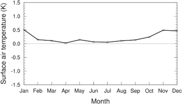
Figure 4. Area-averaged responses in SAT over the Arctic Ocean in response to additional gas-flaring-related BC.
Download figure:
Standard image High-resolution imageBoth meridional heat and moisture transport increased when considering flaring-related BC (supplementary figure S2). The transported energy to the Arctic Ocean was primarily used to promote the melting of Arctic sea ice (July: −1.8%) during summer (figure 5(a)). Consequently, more SW radiation could penetrate the less ice-covered ocean. With the advent of the Arctic cold season, the Arctic Ocean began to release large amounts of energy as turbulent (November: 1.8 W m−2) heat fluxes into the relatively colder atmosphere through the less ice-covered part of the ocean (figure 5(a)) (Serreze et al 2009). The increase in surface turbulence flux through the sea surface increased water vapor, and thus also increased LW radiation. Moreover, this triggered the warming and melting of sea ice, resulting in a positive feedback, which could amplify Arctic warming. The decrease in Arctic sea-ice extent was greatest in November (−2.7%; figure 5(a)).

Figure 5. Zonally-averaged responses to gas-flaring-related BC. (a) Response of the sea-ice fraction (shaded) and surface turbulent (sensible + latent) heat flux (contour). (b) Response of the Arctic Ocean in DLR (black), SAT (red) and total precipitable water (PW) (blue).
Download figure:
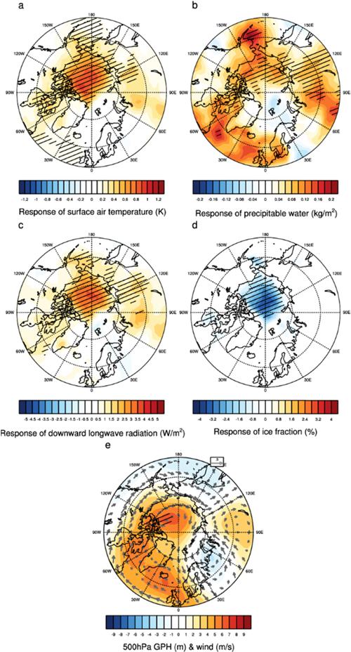
Standard image High-resolution imageThe robust features of the response to flaring-related BC included increased atmospheric water vapor (figure 6(b)), increased surface DLR (figure 6(c)) and decreased sea-ice coverage (figure 6(d)). The enhanced surface DLR is a consequence of increased atmospheric water vapor and warming. During the Arctic cold season, variations in DLR are fundamental for modulating the Arctic surface temperature (Kim and Kim 2017). Monthly SAT responses over the Arctic Ocean (north of 75°N) were highly related to the total PW and DLR, especially during the cold season (figure 5(b)). The enhancement of the PW in the Pacific sector of the Arctic (Chukchi Sea, Bering Sea) seems to be due to the high-pressure anomalies in the Arctic Ocean (figure 6(e)), resulting in an increase in poleward moisture transport.
Figure 6. Response of (a) SAT (unit: K), (b) total PW (unit: kg/m2), (c) DLR flux (unit: W/m2), (d) sea-ice fraction (unit: %), (e) GPH and wind at 500 hPa to updated flaring-related BC emissions during the cold season (October to February). Hatched regions indicate significant differences at the 95% confidence level.
Download figure:
Standard image High-resolution image
Next, we performed additional experiments to gain further confidence of the contribution of local sea-ice feedback to the warming of the Arctic Ocean. Therefore, we conducted the same experimental simulation, but used only the atmospheric model not coupled with the ocean/sea-ice model. Unlike the significant warming over the gas-flaring region in spring (supplementary figure S3), there was no significant warming over the Arctic Ocean during the cold season (supplementary figure S4(a)). These findings confirmed the role of local sea-ice feedback in the increase in cold-season warming shown in figure 6.
BC influences the properties of both ice and liquid clouds through diverse and complex processes (Yoon et al 2016). To examine the indirect effects of flaring-related BC, we calculated the difference in cloud condensation nuclei between the FLARE and CONT cases. Given that there was little difference between these cases, we concluded that the indirect effect of flaring-related BC could be ignored (see supplementary figure S5).
5. Discussion
Our findings imply that a regional change in anthropogenic aerosol forcing is capable of modulating Arctic sea ice in regions far from the aerosol source with a time lag. We determined that increased BC emissions over the pan-Arctic region would result in additional sea-ice melting in the Arctic Ocean through changes in circulation and local sea-ice feedback. BC typically remains in the atmosphere for days to weeks and is thus considered a short-lived climate forcer. In this regard, controlling BC particles through emission reductions would have immediate benefits for air quality and Arctic amplification. Therefore, the World Bank's goal of halting surplus gas flaring in the oil industry by 2030 (Hildén et al 2017) seems appropriate. The results of this study suggest that not only the consumption of energy, but the production process can increase Arctic warming. As such, incorporating BC emissions from gas flaring will contribute to more reliable predictions by improving the accuracy of Arctic climate simulations. Consequently, we recommend that flaring-induced BC should be implemented in future climate projections.
Although the model, which simulated gas-flaring-related BC responses, seems robust, it is worth noting a number of limitations in the model simulations of this study. First, the SOM is not capable of simulating further interactions with the deeper ocean and with dynamic sea ice. Changes in ocean energy advection do not occur in the SOM. Therefore, the cold-season climate changes described here should be interpreted with some caution. In addition, the CAM5 exhibits deficiencies when simulating complex feedback processes involved in the Arctic climate system. Because the combustion processes that emit BC also emit organic carbon (and sulfate aerosols), which has a radiative cooling effect, the full forcing effect of the combustion process is challenging to determine (Evans et al 2017). The highly efficient scavenging of BC by liquid cloud processes (Wang et al 2013) and the coarse horizontal resolution (∼100 km) of the model (Ma et al 2014) are also limitations of this study. Finally, considering the uncertainty of the BC emission data by the gas flaring used in this study (Winiger et al 2017), emission distribution and source attribution in the inventory need improving.
Acknowledgments
This work was supported by the research project of the Korea Polar Research Institute titled 'Development and Application of the Korea Polar Prediction System for Climate Change and Disastrous Weather Events' (PE19130). B-M K was supported by the Korea Meteorological Administration Research and Development Program under Grant KMI2018-01011. S-J J was supported by the National Research Foundation of Korea (NRF) grant funded by the Korea government (MSIT) (NRF-2019R1A2C3002868). R J P and J I J were supported by the National Research Foundation of Korea (NRF) grant funded by the Korea government (MSIT) (NRF-2018R1A5A1024958). J Y was partially supported by GIST Research Institute (GRI) grant funded by the GIST in 2019.
Author contributions
B-M K and S-J J designed the research and wrote the manuscript. M-H C wrote the paper, performed the experiments and analyzed the data. All the authors discussed the results and commented on the manuscript.
Competing financial interests
The authors declare no competing financial interests.